The AutoTune filter

By the Fourier theorem, any price curve is a mix of many long-term and short-term cycles. Once in a while a dominant market cycle emerges and can be exploited for trading. In his TASC 5/2026 article, John Ehlers described an algorithm for detecting such dominant cycles, using them to tune a bandpass filter, and creating a profitable trading system. Here’s how to do it.

Ehlers’ Easylanguage code from the TASC article can be directly converted to C for Zorro.  ChatGPT does the job in a few seconds. First, the cycle detector:

var MinCorr, Filt;
var AutoTune(vars Data,int Window)
{
  Filt = HighPass3(Data,Window);
  vars HP = series(Filt);
  var Corr[256];
  int Lag, J;
  for(Lag = 1; Lag <= Window; Lag++)
  {
    var Sx = 0., Sy = 0.;
    var Sxx = 0., Sxy = 0., Syy = 0.;
    for(J = 0; J < Window; J++)
    {
      var X = HP[J];
      var Y = HP[Lag + J];
      Sx += X; Sy += Y;
      Sxx += X*X; Sxy += X*Y; Syy += Y*Y;
    }
    var Den1 = Window*Sxx - Sx*Sx;
    var Den2 = Window*Syy - Sy*Sy;
    Corr[Lag] = (Window*Sxy - Sx*Sy) / sqrt(fix0(Den1*Den2));
  }

  MinCorr = 1.;
  var DC = Window;
  for(Lag = 1; Lag <= Window; Lag++)
    if(Corr[Lag] < MinCorr) {
      MinCorr = Corr[Lag];
      DC = 2*Lag;
    }

  vars DCs = series(DC,2);
  return DCs[0] = clamp(DC,DCs[1]-2.,DCs[1]+2.);
}

The output of the AutoTune function is supposed to be the dominant price cycle in units of bars. It is then used to set the center frequency of a bandpass filter. Since Zorro has already a bandpass filter in its arsenal, I named Ehlers’ new version BandPass2:

var BandPass2(vars Data, int Period, var Bandwidth)
{
  var L1 = cos(2.*PI/Period);
  var G1 = cos(Bandwidth*2.*PI/Period);
  var S1 = 1./G1 - sqrt(1./(G1*G1) - 1.);
  vars BP = series(0,3);
  return BP[0] = 0.5*(1.-S1)*(Data[0]-Data[2]) 
    + L1*(1.+S1)*BP[1] - S1*BP[2];
}

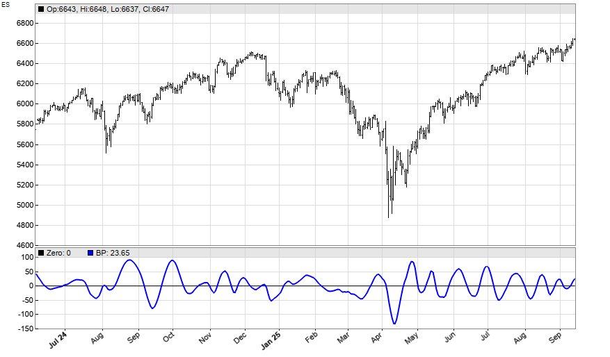
Here’s some code for reproducing Ehlers’ ES chart in the article:

function run()
{
  BarPeriod = 1440;
  StartDate = 2024;
  EndDate = 2025;
  asset("ES");
  var DC = AutoTune(seriesC(),20);
  var BP = BandPass2(seriesC(),DC,0.25);
  plot("Zero",0,NEW,BLACK);
  plot("BP",BP,LINE,BLUE);
}

The resulting chart:

How can we use this bandpass output for a trade signal? Ehlers used the zero crossovers of its rate-of-change (ROC). In this way he generated an impressive equity curve in his article, unfortunately with in-sample optimization. For a more realistic result, we’re using walk-forward analysis and reinvest profits by the square root rule:

function run()
{
  BarPeriod = 1440;
  StartDate = 2010;
  EndDate = 2025;
  Capital = 100000;

  asset("ES");
  set(TESTNOW,PARAMETERS);
  NumWFOCycles = 10;

  int Window = optimize("Window",26,10,30,2);
  var BW = optimize("BW",0.22,0.10,0.30,0.01);
  var Thresh = -optimize("Thresh",0.22,0.1,0.3,0.01);
  var DC = AutoTune(seriesC(),Window);
  var BP = BandPass2(seriesC(),DC,BW);
  vars ROCs = series(BP-ref(BP,2));
  
  Lots = 0.5*(Capital+sqrt(1.+ProfitTotal/Capital))/MarginCost;
  MaxLong = MaxShort = 1;
  if(crossOver(ROCs,0) && MinCorr < Thresh)
    enterLong();
  if(crossUnder(ROCs,0) && MinCorr < Thresh && Filt > 0)
    enterShort();
}

The signals are filtered by a threshold that determines whether we’re in a cyclic market condition or not. The system is not fully symmetrical in long and short positions. Training and testing produced this equity curve:

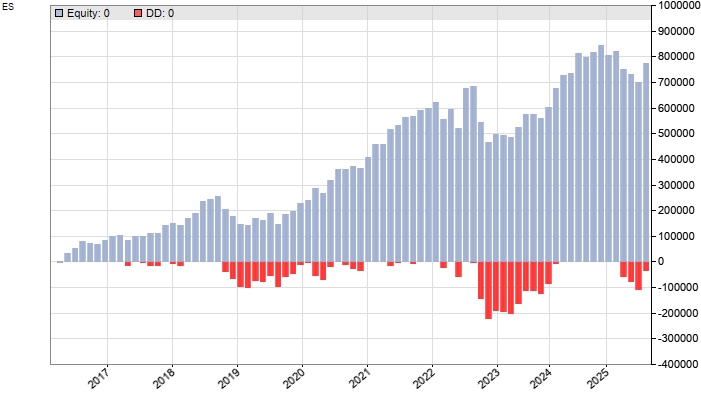
This curve does not look as impressive as Ehler’s one, but the CAGR is in the 25% area, much better than a buy-and-hold strategy. The code can be downloaded from the 2026 script repository.