By the Fourier theorem, any price curve is a mix of many long-term and short-term cycles. Once in a while a dominant market cycle emerges and can be exploited for trading. In his TASC 5/2026 article, John Ehlers described an algorithm for detecting such dominant cycles, using them to tune a bandpass filter, and creating a profitable trading system. Here’s how to do it.
Ehlers’ Easylanguage code from the TASC article can be directly converted to C for Zorro. ChatGPT does the job in a few seconds. First, the cycle detector:
var MinCorr, Filt;
var AutoTune(vars Data,int Window)
{
  Filt = HighPass3(Data,Window);
  vars HP = series(Filt);
  var Corr[256];
  int Lag, J;
  for(Lag = 1; Lag <= Window; Lag++)
  {
    var Sx = 0., Sy = 0.;
    var Sxx = 0., Sxy = 0., Syy = 0.;
    for(J = 0; J < Window; J++)
    {
      var X = HP[J];
      var Y = HP[Lag + J];
      Sx += X; Sy += Y;
      Sxx += X*X; Sxy += X*Y; Syy += Y*Y;
    }
    var Den1 = Window*Sxx - Sx*Sx;
    var Den2 = Window*Syy - Sy*Sy;
    Corr[Lag] = (Window*Sxy - Sx*Sy) / sqrt(fix0(Den1*Den2));
  }

  MinCorr = 1.;
  var DC = Window;
  for(Lag = 1; Lag <= Window; Lag++)
    if(Corr[Lag] < MinCorr) {
      MinCorr = Corr[Lag];
      DC = 2*Lag;
    }

  vars DCs = series(DC,2);
  return DCs[0] = clamp(DC,DCs[1]-2.,DCs[1]+2.);
}
The output of the AutoTune function is supposed to be the dominant price cycle in units of bars. It is then used to set the center frequency of a bandpass filter. Since Zorro has already a bandpass filter in its arsenal, I named Ehlers’ new version BandPass2:
var BandPass2(vars Data, int Period, var Bandwidth)
{
  var L1 = cos(2.*PI/Period);
  var G1 = cos(Bandwidth*2.*PI/Period);
  var S1 = 1./G1 - sqrt(1./(G1*G1) - 1.);
  vars BP = series(0,3);
  return BP[0] = 0.5*(1.-S1)*(Data[0]-Data[2])
    + L1*(1.+S1)*BP[1] - S1*BP[2];
}
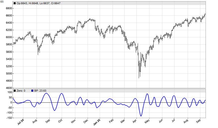
Here’s some code for reproducing Ehlers’ ES chart in the article:
function run()
{
  BarPeriod = 1440;
  StartDate = 2024;
  EndDate = 2025;
  asset("ES");
  var DC = AutoTune(seriesC(),20);
  var BP = BandPass2(seriesC(),DC,0.25);
  plot("Zero",0,NEW,BLACK);
  plot("BP",BP,LINE,BLUE);
}
The resulting chart:
How can we use this bandpass output for a trade signal? Ehlers used the zero crossovers of its rate-of-change (ROC). In this way he generated an impressive equity curve in his article, unfortunately with in-sample optimization. For a more realistic result, we’re using walk-forward analysis and reinvest profits by the square root rule:
function run()
{
  BarPeriod = 1440;
  StartDate = 2010;
  EndDate = 2025;
  Capital = 100000;

  asset("ES");
  set(TESTNOW,PARAMETERS);
  NumWFOCycles = 10;

  int Window = optimize("Window",26,10,30,2);
  var BW = optimize("BW",0.22,0.10,0.30,0.01);
  var Thresh = -optimize("Thresh",0.22,0.1,0.3,0.01);
  var DC = AutoTune(seriesC(),Window);
  var BP = BandPass2(seriesC(),DC,BW);
  vars ROCs = series(BP-ref(BP,2));

  Lots = 0.5*(Capital+sqrt(1.+ProfitTotal/Capital))/MarginCost;
  MaxLong = MaxShort = 1;
  if(crossOver(ROCs,0) && MinCorr < Thresh)
    enterLong();
  if(crossUnder(ROCs,0) && MinCorr < Thresh && Filt > 0)
    enterShort();
}
The signals are filtered by a threshold that determines whether we’re in a cyclic market condition or not. The system is not fully symmetrical in long and short positions. Training and testing produced this equity curve:
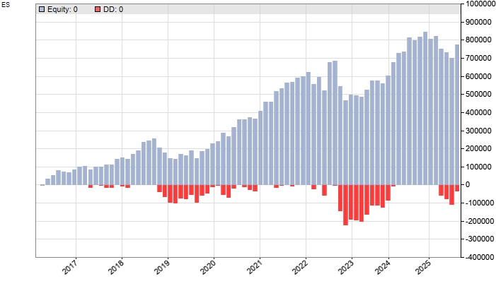
This curve does not look as impressive as Ehler’s one, but the CAGR is in the 25% area, much better than a buy-and-hold strategy. The code can be downloaded from the 2026 script repository.
Thanks for putting the C version out, the EasyLanguage-to-Zorro ports are the part nobody else does, and they’re what makes any of this checkable. ChatGPT still produces bugs, we still need to keep it verified.
One thing I’d add rather than dispute. The AutoTune machinery assumes a dominant cycle is there to be found, and I couldn’t see anywhere in the post where that assumption gets its own test – no shuffled control, no random-period arm. So the 25% is measured against buy-and-hold, but not against “the same filter, tuned to a period that means nothing”.
I ran that premise separately, on hourly bars of three majors, 2000–2026, against a null of the same returns shuffled — which destroys serial structure and leaves the fat tails alone, so a peak that survives is structure and not kurtosis. Two hundred shuffles for the band.
In the returns, nothing stood up: no bin reached 1.2× the 99th percentile of the shuffled band, and about ten bins per instrument cleared it at all, which is what a thousand bins and a 99% band give you by chance. The bins that cleared repeated on no second instrument. Period estimates didn’t survive the move to the next window either — six instrument-estimator cells, all inside ±1.6 sd of shuffled.
The part I’d stress is the positive control, because it’s what stops this being a null from a blunt instrument. In absolute returns a peak stands up enormously — 24 bars at six to twenty-nine times the band on all three, and again at 98 on M15 and 293 on M5. That’s the trading day at each scale. Fed a real cycle, Welch and Burg find it and find it loudly. They just don’t find one in price.
Two honest limits. My A/B was a channel breakout whose only parameter is the lookback, chosen because a second free parameter lets either arm win by tuning rather than by adapting, so it says nothing directly about a band-pass tuned for mean reversion, which asks something different of the same estimate. And your result comes out of walk-forward optimisation, which is the right method; my worry is only that if the period itself isn’t persistent, walk-forward hides that rather than catching it.
Numbers and method are at https://turnmarks.com/filters/adaptive if useful. I’d be glad to be wrong about the premise: a shuffled-period arm on your ES setup would settle it faster than anything I ran.