
Trading systems come in two flavors: model-based and data-mining. This article deals with model based strategies. Even when the basic algorithms are not complex, properly developing them has its difficulties and pitfalls (otherwise anyone would be doing it). A significant market inefficiency gives a system only a relatively small edge. Any little mistake can turn a winning strategy into a losing one. And you will not necessarily notice this in the backtest.
Developing a model-based strategy begins with the market inefficiency that you want to exploit. The inefficiency produces a price anomaly or price pattern that you can describe with a qualitative or quantitative model. Such a model predicts the current price yt from the previous price yt-1 plus some function f of a limited number of previous prices plus some noise term ε:
[pmath size=16]y_t ~=~ y_{t-1} + f(y_{t-1},~…, ~y_{t-n}) + epsilon[/pmath]
The time distance between the prices yt is the time frame of the model; the number n of prices used in the function f is the lookback period of the model. The higher the predictive f term in relation to the nonpredictive ε term, the better is the strategy. Some traders claim that their favorite method does not predict, but ‘reacts on the market’ or achieves a positive return by some other means. On a certain trader forum you can even encounter a math professor who re-invented the grid trading system, and praised it as non-predictive and even able to trade a random walk curve. But systems that do not predict yt in some way must rely on luck; they only can redistribute risk, for instance exchange a high risk of a small loss for a low risk of a high loss. The profit expectancy stays negative. As far as I know, the professor is still trying to sell his grid trader, still advertising it as non-predictive, and still regularly blowing his demo account with it.
Trading by throwing a coin loses the transaction costs. But trading by applying the wrong model – for instance, trend following to a mean reverting price series – can cause much higher losses. The average trader indeed loses more than by random trading (about 13 pips per trade according to FXCM statistics). So it’s not sufficient to have a model; you must also prove that it is valid for the market you trade, at the time you trade, and with the used time frame and lookback period.
Not all price anomalies can be exploited. Limiting stock prices to 1/16 fractions of a dollar is clearly an inefficiency, but it’s probably difficult to use it for prediction or make money from it. The working model-based strategies that I know, either from theory or because we’ve been contracted to code some of them, can be classified in several categories. The most frequent are:
1. Trend
Momentum in the price curve is probably the most significant and most exploited anomaly. No need to elaborate here, as trend following was the topic of a whole article series on this blog. There are many methods of trend following, the classic being a moving average crossover. This ‘hello world’ of strategies (here the scripts in R and in C) routinely fails, as it does not distinguish between real momentum and random peaks or valleys in the price curve.
The problem: momentum does not exist in all markets all the time. Any asset can have long non-trending periods. And contrary to popular belief this is not necessarily a ‘sidewards market’. A random walk curve can go up and down and still has zero momentum. Therefore, some good filter that detects the real market regime is essential for trend following systems. Here’s a minimal Zorro strategy that uses a lowpass filter for detecting trend reversal, and the MMI indicator for determining when we’re entering trend regime:
function run()
{
  vars Price = series(price());
  vars Trend = series(LowPass(Price,500));

  vars MMI_Raw = series(MMI(Price,300));
  vars MMI_Smooth = series(LowPass(MMI_Raw,500));

  if(falling(MMI_Smooth)) {
    if(valley(Trend))
      reverseLong(1);
    else if(peak(Trend))
      reverseShort(1);
  }
}
The profit curve of this strategy:
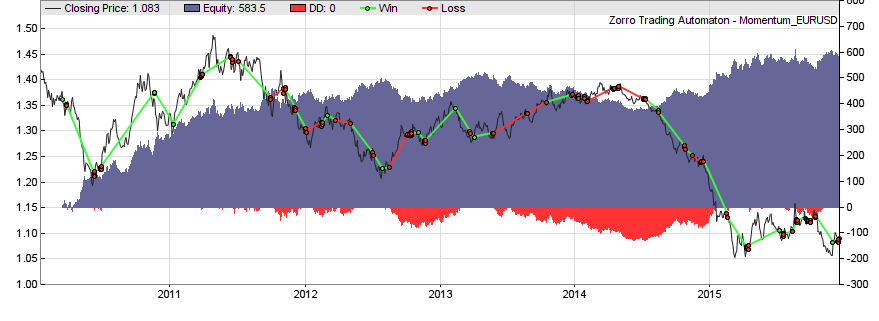
(For the sake of simplicity all strategy snippets on this page are barebone systems with no exit mechanism other than reversal, and no stops, trailing, parameter training, money management, or other gimmicks. Of course the backtests mean in no way that those are profitable systems. The P&L curves are all from EUR/USD, an asset good for demonstrations since it seems to contain a little bit of every possible inefficiency).
2. Mean reversion
A mean reverting market believes in a ‘real value’ or ‘fair price’ of an asset. Traders buy when the actual price is cheaper than it ought to be in their opinion, and sell when it is more expensive. This causes the price curve to revert back to the mean more often than in a random walk. Random data are mean reverting 75% of the time (proof here), so anything above 75% is caused by a market inefficiency. A model:
[pmath size=16]y_t ~=~ y_{t-1} ~-~ 1/{1+lambda}(y_{t-1}- hat{y}) ~+~ epsilon[/pmath]
[pmath size=16]y_t[/pmath] = price at bar t
[pmath size=16]hat{y}[/pmath] = fair price
[pmath size=16]lambda[/pmath] = half-life factor
[pmath size=16]epsilon[/pmath] = some random noise term
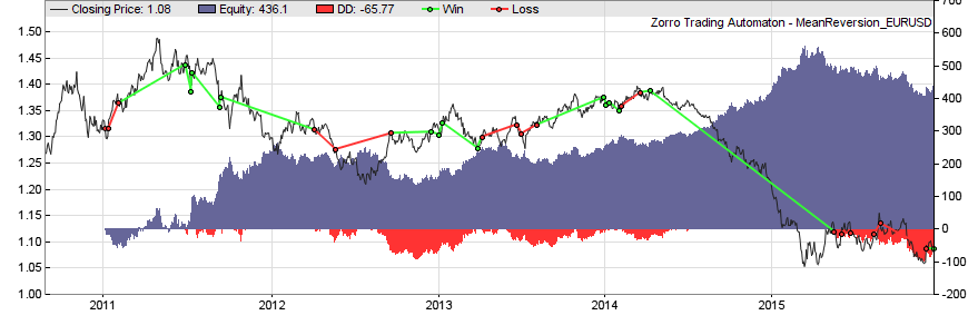
The higher the half-life factor, the weaker is the mean reversion. The half-life of mean reversion in price series ist normally in the range of 50-200 bars. You can calculate λ by linear regression between yt-1 and (yt-1-yt). The price series need not be stationary for experiencing mean reversion, since the fair price is allowed to drift. It just must drift less as in a random walk. Mean reversion is usually exploited by removing the trend from the price curve and normalizing the result. This produces an oscillating signal that can trigger trades when it approaches a top or bottom. Here’s the script of a simple mean reversion system:
function run()
{
  vars Price = series(price());
  vars Filtered = series(HighPass(Price,30));
  vars Signal = series(FisherN(Filtered,500));
  var Threshold = 1.0;

  if(Hurst(Price,500) < 0.5) { // do we have mean reversion?
    if(crossUnder(Signal,-Threshold))
      reverseLong(1);
    else if(crossOver(Signal,Threshold))
      reverseShort(1);
  }
}
The highpass filter dampens all cycles above 30 bars and thus removes the trend from the price curve. The result is normalized by the Fisher transformation which produces a Gaussian distribution of the data. This allows us to determine fixed thresholds at 1 and -1 for separating the tails from the resulting bell curve. If the price enters a tail in any direction, a trade is triggered in anticipation that it will soon return into the bell’s belly. For detecting mean reverting regime, the script uses the Hurst Exponent. The exponent is 0.5 for a random walk. Above 0.5 begins momentum regime and below 0.5 mean reversion regime.
3. Statistical Arbitrage
Strategies can exploit the similarity between two or more assets. This allows to hedge the first asset by a reverse position in the second asset, and this way derive profit from mean reversion of their price difference:
[pmath size=16]y ~=~ h_1 y_1 – h_2 y_2[/pmath]
where y1 and y2 are the prices of the two assets and the multiplication factors h1 and h2 their hedge ratios. The hedge ratios are calculated in a way that the mean of the difference y is zero or a constant value. The simplest method for calculating the hedge ratios is linear regression between y1 and y2. A mean reversion strategy as above can then be applied to y.
The assets need not be of the same type; a typical arbitrage system can be based on the price difference between an index ETF and its major stock. When y is not stationary – meaning that its mean tends to wander off slowly – the hedge ratios must be adapted in real time for compensating. Here is a proposal using a Kalman Filter by a fellow blogger.
The simple arbitrage system from the R tutorial:
require(quantmod)

symbols <- c("AAPL", "QQQ")
getSymbols(symbols)

#define training set
startT  <- "2007-01-01"
endT    <- "2009-01-01"
rangeT  <- paste(startT,"::",endT,sep ="")
tAAPL   <- AAPL[,6][rangeT]
tQQQ   <- QQQ[,6][rangeT]

#compute price differences on in-sample data
pdtAAPL <- diff(tAAPL)[-1]
pdtQQQ <- diff(tQQQ)[-1]

#build the model
model  <- lm(pdtAAPL ~ pdtQQQ - 1)

#extract the hedge ratio (h1 is assumed 1)
h2 <- as.numeric(model$coefficients[1])

#spread price (in-sample)
spreadT <- tAAPL - h2 * tQQQ

#compute statistics of the spread
meanT    <- as.numeric(mean(spreadT,na.rm=TRUE))
sdT      <- as.numeric(sd(spreadT,na.rm=TRUE))
upperThr <- meanT + 1 * sdT
lowerThr <- meanT - 1 * sdT

#run in-sample test
spreadL  <- length(spreadT)
pricesB  <- c(rep(NA,spreadL))
pricesS  <- c(rep(NA,spreadL))
sp       <- as.numeric(spreadT)
tradeQty <- 100
totalP   <- 0

for(i in 1:spreadL) {
     spTemp <- sp[i]
     if(spTemp < lowerThr) {
        if(totalP <= 0){
           totalP     <- totalP + tradeQty
           pricesB[i] <- spTemp
        }
     } else if(spTemp > upperThr) {
       if(totalP >= 0){
          totalP <- totalP - tradeQty
          pricesS[i] <- spTemp
       }
    }
}
4. Price constraints
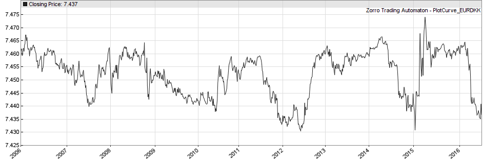
A price constraint is an artificial force that causes a constant price drift or establishes a price range, floor, or ceiling. The most famous example was the EUR/CHF price cap mentioned in the first part of this series. But even after removal of the cap, the EUR/CHF price has still a constraint, this time not enforced by the national bank, but by the current strong asymmetry in EUR and CHF buying power. An extreme example of a ranging price is the EUR/DKK pair (see below). All such constraints can be used in strategies to the trader’s advantage.
5. Cycles
Non-seasonal cycles are caused by feedback from the price curve. When traders believe in a ‘fair price’ of an asset, they often sell or buy a position when the price reaches a certain distance from that value, in hope of a reversal. Or they close winning positions when the favorite price movement begins to decelerate. Such effects can synchronize entries and exits among a large number of traders, and cause the price curve to oscillate with a period that is stable over several cycles. Often many such cycles are superposed on the curve, like this:
[pmath size=16]y_t ~=~ hat{y} ~+~ sum{i}{}{a_i sin(2 pi t/C_i+D_i)} ~+~ epsilon[/pmath]
When you know the period Ci and the phase Di of the dominant cycle, you can calculate the optimal trade entry and exit points as long as the cycle persists. Cycles in the price curve can be detected with spectral analysis functions – for instance, fast Fourier transformation (FFT) or simply a bank of narrow bandpass filters. Here is the frequency spectrum of the EUR/USD in October 2015:

Exploiting cycles is a little more tricky than trend following or mean reversion. You need not only the cycle length of the dominant cycle of the spectrum, but also its phase (for triggering trades at the right moment) and its amplitude (for determining if there is a cycle worth trading at all). This is a barebone script:
function run()
{
  vars Price = series(price());
  var Phase = DominantPhase(Price,10);
  vars Signal = series(sin(Phase+PI/4));
  vars Dominant = series(BandPass(Price,rDominantPeriod,1));
  ExitTime = 10*rDominantPeriod;
  var Threshold = 1*PIP;

  if(Amplitude(Dominant,100) > Threshold) {
    if(valley(Signal))
      reverseLong(1);
    else if(peak(Signal))
      reverseShort(1);
  }
}
The DominantPhase function determines both the phase and the cycle length of the dominant peak in the spectrum; the latter is stored in the rDominantPeriod variable. The phase is converted to a sine curve that is shifted ahead by π/4. With this trick we’ll get a sine curve that runs ahead of the price curve. Thus we do real price prediction here, only question is if the price will follow our prediction. This is determined by applying a bandpass filter centered at the dominant cycle to the price curve, and measuring its amplitude (the ai in the formula). If the amplitude is above a threshold, we conclude that we have a strong enough cycle. The script then enters long on a valley of the run-ahead sine curve, and short on a peak. Since cycles are shortlived, the duration of a trade is limited by ExitTime to a maximum of 10 cycles.
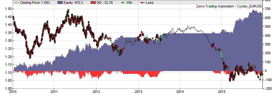
We can see from the P&L curve that there were long periods in 2012 and 2014 with no strong cycles in the EUR/USD price curve.
6. Clusters
The same effect that causes prices to oscillate can also let them cluster at certain levels. Extreme clustering can even produce “supply” and “demand” lines (also known as “support and resistance“), the favorite subjects in trading seminars. Expert seminar lecturers can draw support and resistance lines on any chart, no matter if it’s pork belly prices or last year’s baseball scores. However the mere existence of those lines remains debatable: There are few strategies that really identify and exploit them, and even less that really produce profits. Still, clusters in price curves are real and can be easily identified in a histogram similar to the cycles spectogram.
7. Curve patterns
They arise from repetitive behavior of traders. Traders not only produce, but also believe in many curve patterns; most – such as the famous ‘head and shoulders’ pattern that is said to predict trend reversal – are myths (at least I have not found any statistical evidence of it, and heard of no other any research that ever confirmed the existence of predictive heads and shoulders in price curves). But some patterns, for instance “cups” or “half-cups”, really exist and can indeed precede an upwards or downwards movement. Curve patterns – not to be confused with candle patterns – can be exploited by pattern-detecting methods such as the Fréchet algorithm.
A special variant of a curve pattern is the Breakout – a sudden momentum after a long sidewards movement. Is can be caused, for instance, by trader’s tendency to place their stop losses as a short distance below or above the current plateau. Triggering the first stops then accelerates the price movement until more and more stops are triggered. Such an effect can be exploited by a system that detects a sidewards period and then lies in wait for the first move in any direction.
8. Seasonality
“Season” does not necessarily mean a season of a year. Supply and demand can also follow monthly, weekly, or daily patterns that can be detected and exploited by strategies. For instance, the S&P500 index is said to often move upwards in the first days of a month, or to show an upwards trend in the early morning hours before the main trading session of the day. Since seasonal effects are easy to exploit, they are often shortlived, weak, and therefore hard to detect by just eyeballing price curves. But they can be found by plotting a day, week, or month profile of average price curve differences.
9. Gaps
When market participants contemplate whether to enter or close a position, they seem to come to rather similar conclusions when they have time to think it over at night or during the weekend. This can cause the price to start at a different level when the market opens again. Overnight or weekend price gaps are often more predictable than price changes during trading hours. And of course they can be exploited in a strategy. On the Zorro forum was recently a discussion about the “One Night Stand System“, a simple currency weekend-gap trader with mysterious profits.
10. Autoregression and heteroskedasticity
The latter is a fancy word for: “Prices jitter a lot and the jittering varies over time”. The ARIMA and GARCH models are the first models that you encounter in financial math. They assume that future returns or future volatility can be determined with a linear combination of past returns or past volatility. Those models are often considered purely theoretical and of no practical use. Not true: You can use them for predicting tomorrow’s price just as any other model. You can examine a correlogram – a statistics of the correlation of the current return with the returns of the previous bars – for finding out if an ARIMA model fits to a certain price series. Here are two excellent articles by fellow bloggers for using those models in trading strategies: ARIMA+GARCH Trading Strategy on the S&P500 and Are ARIMA/GARCH Predictions Profitable?
11. Price shocks
Price shocks often happen on Monday or Friday morning when companies or organizations publish good or bad news that affect the market. Even without knowing the news, a strategy can detect the first price reactions and quickly jump onto the bandwagon. This is especially easy when a large shock is shaking the markets. Here’s a simple Forex portfolio strategy that evaluates the relative strengths of currencies for detecting price shocks:
function run()
{
  BarPeriod = 60;
  ccyReset();
  string Name;
  while(Name = (loop(Assets)))
  {
    if(assetType(Name) != FOREX)
      continue; // Currency pairs only
    asset(Name);
    vars Prices = series(priceClose());
    ccySet(ROC(Prices,1)); // store price change as strength
  }

// get currency pairs with highest and lowest strength difference
  string Best = ccyMax(), Worst = ccyMin();
  var Threshold = 1.0; // The shock level

  static char OldBest[8], OldWorst[8];	// static for keeping contents between runs
  if(*OldBest && !strstr(Best,OldBest)) { // new strongest asset?
    asset(OldBest);
    exitLong();
    if(ccyStrength(Best) > Threshold) {
      asset(Best);
      enterLong();
    }
  }
  if(*OldWorst && !strstr(Worst,OldWorst)) { // new weakest asset?
    asset(OldWorst);
    exitShort();
    if(ccyStrength(Worst) < -Threshold) {
      asset(Worst);
      enterShort();
    }
  }

// store previous strongest and weakest asset names
  strcpy(OldBest,Best);
  strcpy(OldWorst,Worst);
}
The equity curve of the currency strength system (you’ll need Zorro 1.48 or above):
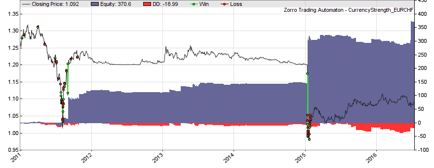
The blue equity curve above reflects profits from small and large jumps of currency prices. You can clearly identify the Brexit and the CHF price cap shock. Of course such strategies would work even better if the news could be early detected and interpreted in some way. Some data services provide news events with a binary valuation, like “good” or “bad”. Especially of interest are earnings reports, as provided by data services such as Zacks or Xignite. Depending on which surprises the earnings report contains, stock prices and implied volatilities can rise or drop sharply at the report day, and generate quick profits.
For learning what can happen when news are used in more creative ways, I recommend the excellent Fear Index by Robert Harris – a mandatory book in any financial hacker’s library.
This was the second part of the Build Better Strategies series. The third part will deal with the process to develop a model-based strategy, from inital research up to building the user interface. In case someone wants to experiment with the code snippets posted here, I’ve added them to the 2015 scripts repository. They are no real strategies, though. The missing elements – parameter optimization, exit algorithms, money management etc. – will be the topic of the next part of the series.
Keep it coming, love your articles.
Is this ‘dominant cycle’ idea similar to Ehlers’ work on the subject?
I don’t seem to recall any mention of determining the amplitude of the cycle as a filter for removing weak/noise trades. Interesting! Will have to look at that. Thanks for the post.
Yes, the dominant cycle concept is from Ehlers. In my experience, a filter that detects the market situation, like the amplitude threshold, is essential for most model based strategies – it’s almost more important than the trade algorithm itself.
Jcl, would you care to explain/comment further the amplitude indicator that runs in Zorro? John Ehlers work is really great, but seeing applied to real markets nowadays is even more valuable, IMHO.
Thanks a lot
Best
From the Zorro manual, the Aplitude is “the highest high minus the lowest low of the Data series, smoothed over the TimePeriod with an EMA so that the more recent fluctuations become more weight. “. So I think it’s simply something like EMA(range,timeperiod) of the frequency band of the dominant cycle.
Hi
I cant reproduce any of the results above. I guess it is due to trailing and similar parameters. In the same way, maybe I am coding a strategy which make sense but at the end I forget it because I see it as non profitable when the problem is due to the money management and risk control.
Would not be useful to add a workshop where some risk management ideas are implemented so that beginners can get better understanding of it and develop better strategies. I know there is all those trailing functions built on but to use one or another until one gets a nice curve is like walking half blind, or like throwing a coin hoping that the next function tried will work.
Forget about risk management at this point. It would just distort results and is useless when the algorithm has no edge. First step is the model. Second step is an algorithm based on that model, with a positive return on a simulation with realistic trading cost. This is done in the examples above. It is quite easy to come up with such systems that seemingly produce good returns. The hard part is testing if the return is for real or just curve fitting bias. That would be the next step, and only if the system passes that test, the model is justified. Then you can think about making a real strategy from it, with trailing, risk management, money management, and so on. This is the very last step of strategy development, not the first.
Reproducing published results is often difficult, but should not be a problem here. You got the code and the test environment, so you can see what the functions return and which trades are opened. Compare with your own results. This way you can quickly find out where and why they are different.
Hi
Thanks for the fast answer. My fault: I was actually using the assetlist from another broker and the results were completly down. Thats why I thought that there was some magic added to get the results. When I use the fxcm settings I get similar results.
Yes, I read in the manual how a strategy should be develop from basic idea and step by step adding features.
It is difficult to know if there is an edge in the results. There is no a rule like: if the simple idea gives a certain amount of pips then it may have an edge.
Thanks a lot for all these articles icl, I’m reading them like a fascinating book!
Hi jcl,
Can you teach me a bit more about the lambda of the mean reversion, i.e., “You can calculate λ by linear regression between yt-1 and (yt-1-yt)”? Why is that? How can we use lambda in the mean reversion example?
Thank you.
When you reformulate the mean reversion formula above, like this:
y(t) – y(t-1) = a * (y(t-1) – Mean) + Epsilon,
you can see that it is a line equation in the form y = a*x + b, where a = -1/(1+Lambda). When a is nonzero, the price change y(t)-y(t-1) has a linear relationship to the deviation of the previous price from the fair price, y(t-1)-Mean. The mathematical method to determine the slope a from many data pairs ( y(t)-y(t-1), y(t-1)-Mean ) is linear regression. From a you get the half-life parameter Lambda. The market is mean reversing when a is negative.
Thanks for the detail, jcl. It helps a lot.
Hi jcl
Does the procedure look correct to you ?
The steps are as follows:
1. Set our price close lagged by -1 day.
2. Subtract todays price close against yesterdays lagged close
3. Subtract (yesterday price close) – mean(of the -1 lagged price close )
4. Perform a linear regression on (todays price – yesterdays price) ~ (yesterday price close) – mean(of the -1 lagged price close )
R code for this is below, does it look correct?
# Half Life of Mean Reversion
# Andrew Bannerman 9.24.2017
# Random Data
random.data <- c(runif(1500, min=0, max=100))
# Calculate yt-1 and (yt-1-yt)
y.lag <- c(random.data[2:length(random.data)], 0)
y.diff <- random.data – y.lag
prev.y.mean <- y.lag – mean(y.lag)
final <- merge(y.diff, prev.y.mean)
final.df <- as.data.frame(final)
# Linear Regression
result <- lm(y.diff ~ prev.y.mean, data = final.df)
half_life <- -log(2)/coef(result)[2]
half_life
The steps look correct. For the R code I dare not judge the correctness – put in some data and check if the half life value makes sense.
My next question is, can this be applied to a linear trend? I tested the above procedure on the SPY from inception to present and the half life was 939.6574. Doesnt look to correct even thought the procedure looks correct. Jc – have you obtained accurate results using this half life method?
I have, and yes, it can be applied to a trending asset, especially to SPY. But when it trends, check how you calculate the mean: this is your mean reversion target. Use 20 days or so. If you use all the data for the mean, then you might get the half life of SPY reverting to its price of 1980, and I guess that’s infinity.
If you’re interested in this method, get the book by Ernie Chan. It contains a in depth description of mean reverting algos and half life calculation.
Ok if i did present to 20 days, that gives me the half life of the previous 2o days? What about the rest of the sample size? Do we then roll this on a 20 day basis from inception to present? Does it mean the half life is likely to change as the series rolls into the future?
Sure, you must roll. For trading you want the mean and halflife from today, not from 10 years ago. Since price series are nonstationary, the mean changes all the time. The halflife is much more stationary, but it can also change under different market conditions.
First of all, thank you for this blog . I wish I had come across it years ago.
I’m a very unsophisticated (it turns out) options trader. I made my living doing volatility arbitrage, but that game is finished. I’ve been trying to teach myself new trades and I tried pairs trading using some highly correlated index futures. I would do well for a time, but then the spread between the futures would move to a new level usually wiping out whatever profits I had.
I learned that this was because of something called stationarity. Whenever the spread would start trending I would lose.
In your Stat Arb section above you state; ” When y is not stationary – meaning that its mean tends to wander off slowly – the hedge ratios must be adapted in real time for compensating.”
Do you think my problem might be solved by using a Kalman filter as suggested, to come up with dynamic hedge ratios? Would the hedge ratio change fast enough during real time trading to save me?
I was trading these pairs intraday.
thank you
You can use a Kalman filter for almost anything, but for adapting the hedge ratio there are also simpler methods, such as permanent linear regression of the previous N price pairs. The hedge ratio is then the linear regression slope.
I believe the link for the blog post on Kalman filter changed:
https://mktstk.com/2015/08/19/the-kalman-filter-and-pairs-trading/
Being very new on Zorro/R, what’s the easiest but logical way to apply this filter into pair trading?
Thanks for the link. With R, there are Kalman filters in the FKF, KFAS, and several other packages. I have no ready code, but the usage is described in the pdf manuals to the packages.
For anyone interested , I saw a tutorial comparing Copula vs Cointegration in Pairs Trading
here: https://www.quantconnect.com/tutorials/pairs-trading-strategy/
They conclude that Copula method is better
I’m trying to do an intraday pairs trade between two highly correlated/cointegrated futures by hand. I thought I was on to something great but I realize one of the futures contracts has a constant $20-40 difference between bid and ask…..and the other has a $12.50 difference.
If I hit bids and take offers every trade, my profit is completely lost
Am I now unknowingly in the High Frequency business? By that I mean…do I now need an algorithm that bids/offers/cancels within split seconds to lock in the edge I see?
If that is true, can I as an individual trader compete even with an algo , with the big guys? Both contracts trade at the CME….ES and EMD (S&P 500 and 400)
I guess this is related in some ways to your story of setting up a server in Ohio to so ES/SPY arb
thanks again for your patience and insight
Would you be able to show your python code for Signal Processing I can’t find any examples online for finance. I’m a little unsure of how to apply Signal Processing to time series data.
Could you explain a little more how you apply the highness filter to the price?
Highpass filters remove long-term trend from a price curve, including the stationary mean. The result is a curve that oscillates around zero with the same short-term fluctuations that the price curve has.
Much easier than describing this in words is it to just apply a filter and experiment with it. Zorro has a script “Filtertest” or similar that you can use for playing with filters.
Hi, I was wondering what was meant by series(HighPass(Price,30)) & series(FisherN(Filtered,500)) in the Mean Reversion strategy. My interpretation is
The HighPass filter is being calculated based on the last 30 periods of data with the most recent datapoint being stored.
The Fisher Transform is calculated using the last 500 HighPass filter datapoints and trade are taken based on this number.
Yes, that interpretation is correct. There’s a chapter about high pass filter strategies in the Black Book, also John Ehlers has written about them in his books.
Hi,
I would like to better understand the bandpass and fisherN functions but I cannot retrieve the Zorro codes of these functions. Where can I find them?
Thanks,
Romuald
I believe the FisherN source is in the indicators source file. The bandpass source is not, but you can find examples of bandpass filters in the books by John Ehlers.
I am very interested in better understanding the Zorro Z9 script. It is labelled “Dual Momentum Sector Rotation”, however it appears to be doing quite a bit more than described in Gary Antonacci’s book “Dual Momentum Investing”, which barely touches on any details. I have also checked out some of his research papers but have not yet found any that address this. I have used Zorro to develop a basic version of what I understand Gary Antonacci intended, but it selects a single asset at a time …. and it does not work well yet. I do see that Z9 is selecting not a single asset to invest in, but multiple. In that regard it appears to be similar to the algorithm you describe for Z12. I wish to better understand what the algorithm behind Z9 does before I use it. I am a Zorro user with a “S” license.
I trust that this is a reasonable place to present my question. If not please advise.
Sincerely,
Zan Wilson
I haven’t written the Z9 system, but know how it works. Main difference to Antonacci is that it trades a portfolio. Assets are ranked and sorted by their dual momentum and the highest ranking assets are traded. Position sizes are determined by relative momentums. There is also a filtering mechanism in place that increases treasure positions when the market tanks.
I believe someone on the Zorro user forum has replicated Z9 to some extent, you could check out his code.
I have been experimenting with the mean reversion strategy posted on this page. I have been having trouble finding the right threshold for the fisher transform as the numbers increase/decrease based on the volatility of my asset. I was wondering what ways there were to mitigate this issue when using the fisher transform.
Would it be beneficial to fin the p-value of the fisher transform with the Pearson correlation coefficient or am I not approaching the problem correctly?
The threshold is normally not very dependent on volatility since the Fisher transform transfers data to the +-1 range. But it could make sense to slightly optimize the threshold between 0.9 to 1.5 or so, for adjusting the number of trades that the system opens.
For FisherN, Zorro uses
// normalize a value to the -1..+1 range
var Normalize(var* Data,int Period)
{
Period = Max(2,Period);
var vMin = MinVal(Data,Period);
var vMax = MaxVal(Data,Period);
if(vMax>vMin)
return 2.*(*Data-vMin)/(vMax-vMin) – 1.;
else return 0.;
}
Why do we normalize as 2*(x-xmin)/(xmax-xmin)-1 instead of just (x-xmean)/sigma
MeanReversion feature including days since peak and valley show very low predictability in ML models. The highest from this was 0.523
very disappointed
Same with ExploitCycles that had a highest of 0.516
in real world on Cross-validated data, these have lower predictability than FMA or SMA also
Ehler’s methods seem overhyped with heavy overfit. No wonder he is doing more workshops than trading
jcl,
I know this is a dated post but – with the price shocks strategy and currency strength functions:
– how many currency pairs can be used/processed?
– Is there any special setup to backtesting using the currency strength functions (separate assets file? all currency pair data present?)
There is no limit to the currency pairs, and backtesting needs no special setup. But you need historical price data of all pairs in your list.
For the ‘Cycles’ model, could you explain why you add PI/4 to phase of the sine function? Say if Prices follows exactly that of a Sine function, would you keep the phase unchanged, since the sine function is already model the Prices correctly. Thanks.
Because we want to run ahead of the phase. We want to catch the cycle before it actually happens.