
In TASC 3/24, John Ehlers presented several functions for smoothing a price curve without lag, smoothing it even more, and applying a highpass and bandpass filter. No-lag smoothing, highpass, and bandpass filters are already available in the indicator library of the Zorro platform, but not Ehlers’ latest invention, the Ultimate Smoother. It achieves its tremendous smoothing power by subtracting the high frequency components from the price curve, using a highpass filter.
The function below is a straightforward conversion of Ehlers’ EasyLanguage code to C:
var UltimateSmoother (var *Data, int Length)
{
  var f = (1.414*PI) / Length;
  var a1 = exp(-f);
  var c2 = 2*a1*cos(f);
  var c3 = -a1*a1;
  var c1 = (1+c2-c3)/4;
  vars US = series(*Data,4);
  return US[0] = (1-c1)*Data[0] + (2*c1-c2)*Data[1] - (c1+c3)*Data[2]
+ c2*US[1] + c3*US[2];
}
For comparing lag and smoothing power, we apply the ultimate smoother, the super smoother from Zorro’s indicator library, and a standard EMA to an ES chart from 2023:
void run()
{
  BarPeriod = 1440;
  StartDate = 20230201;
  EndDate = 20231201;
  assetAdd("ES","YAHOO:ES=F");
  asset("ES");
  int Length = 30;
  plot("UltSmooth", UltimateSmoother(seriesC(),Length),LINE,MAGENTA);
  plot("Smooth",Smooth(seriesC(),Length),LINE,RED);
  plot("EMA",EMA(seriesC(),3./Length),LINE,BLUE);}
}
The resulting chart replicates the ES chart in the article. The EMA is shown in blue, the super smoothing filter in red, and the ultimate smoother in magenta:

We can see that the ultimate smoother produces indeed the best, albeit smoothed, representation of the price curve.
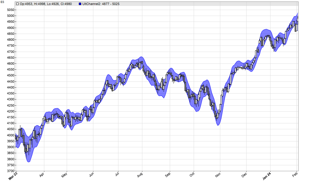
In TASC 4/24, Ehlers also presented two band indicators based on his Ultimate Smoother. Band indicators can be used to trigger long or short positions when the price hits the upper or lower band. The first band indicator, the Ultimate Channel, is again a straightforward conversion to the C language from Ehlers’ TradeStation code:
var UltimateChannel(int Length,int STRLength,int NumSTRs)
{
  var TH = max(priceC(1),priceH());
  var TL = min(priceC(1),priceL());
  var STR = UltimateSmoother(series(TH-TL),STRLength);
  var Center = UltimateSmoother(seriesC(),Length);
  rRealUpperBand = Center + NumSTRs*STR;
  rRealLowerBand = Center - NumSTRs*STR;
  return Center;
}
rRealUpperBand and rRealLowerBand are pre-defined global variables that are used by band indicators in the indicator library of the Zorro platform. For testing the new indicator, we apply it to an ES chart:
void run()
{
  BarPeriod = 1440;
  StartDate = 20230301;
  EndDate = 20240201;
  assetAdd("ES","YAHOO:ES=F");
  asset("ES");
  UltimateChannel(20,20,1);
  plot("UltChannel1",rRealUpperBand,BAND1,BLUE);
  plot("UltChannel2",rRealLowerBand,BAND2,BLUE|TRANSP);
}
The resulting chart replicates the ES chart in Ehlers’ article:
The second band indicator, Ultimate Bands, requires less code than Ehlers’ implementation, since lite-C can apply functions to a whole data series:
var UltimateBands(int Length,int NumSDs)
{
  var Center = UltimateSmoother(seriesC(),Length);
  vars Diffs = series(priceC()-Center);
  var SD = sqrt(SumSq(Diffs,Length)/Length);
  rRealUpperBand = Center + NumSDs*SD;
  rRealLowerBand = Center - NumSDs*SD; return Center;
}
Again applied to the ES chart:
void run()
{
  BarPeriod = 1440;
  StartDate = 20230301;
  EndDate = 20240201;
  assetAdd("ES","YAHOO:ES=F");
  asset("ES");
  UltimateBands(20,1);
  plot("UltBands1",rRealUpperBand,BAND1,BLUE);
  plot("UltBands2",rRealLowerBand,BAND2,BLUE|TRANSP);
}
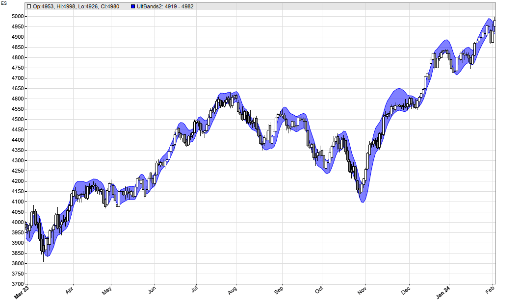
We can see that both indicators produce relatively similar bands with low lag. The code of the Ultimate Smoother and the bands can be downloaded from the 2024 script repository.
Petra, did you run any backtests on this? Eyeballing the crossovers between the super and ultimate smoothers (on this very short time series) it looks like a remarkable success rate for being long when ultimate is higher than super and short when ultimate is below.
Nope. But go ahead and test it – you need only a few lines more in the run function.
Yeah, no, I’m not a Zorro user, I’d have to convert it to R first. I just like reading your articles, they’re consistently good. I’ll post back with my findings if I do convert it, your code is always quite readable, shouldn’t be too hard.
Hi Petra, have some questions about series() in Zorro, as I try to run this in R. I think that this line:
vars US = series(*Data,4);
creates a structure wherein *Data is lagged up to 4 times, so
US[0] = unlagged *Data
US[1] = lagged *Data 1 period
US[2] = lagged *Data 2 period
US[3] = lagged *Data 3 periods
I can do that in R (manual lagging of data series), and have but what I don’t understand is what Data[0], Data[1] and Data[2] represent in the return line? Your code doesn’t use a series() function to make a Data series other than US[], so I can’t see it in your code.
Here’s what I have so far (in R):
USmoo <- function (data, length)
{
f <- (1.414*pi) / length;
a1 <- exp(-f);
c2 <- 2*a1*cos(f);
c3 <- -a1*a1;
c1 <- (1+c2-c3)/4;
#US <- series(data,4); #this is a lagged series, so we'll do some lags
US1 <- stats::lag(data,1)
US2 <- stats::lag(data,2)
#unsure about Data[1] and Data[2]. My guess is certainly wrong, you would have used US[] instead.
DA1 <- stats::lag(data,1)
DA2 <- stats::lag(data,2)
# (your code) return US[0] = (1-c1)*Data[0] + (2*c1-c2)*Data[1] – (c1+c3)*Data[2] + c2*US[1] + c3*US[2];
# my return line wraps with na.omit() to omit NA values
return ( na.omit( (1-c1)*data + (2*c1-c2)*DA1 – (c1+c3)*DA2 + c2*US1 + c3*US2 ) );
}
Down to the lags and return line, it was very easy conversion. Right now Data[1] and Data[2] are identical to US[1] and US[2], reflecting my lack of understanding of what the Data[] series represents. Any thoughts greatly appreciated, from you or other visitors of course.
oh, look here, lots of code samples. I should be able to figure it out.
https://traders.com/Documentation/FEEDbk_docs/2024/04/TradersTips.html
series(X,4) creates a time series of length 4 with the content of X. X[n] is X lagged by n periods. In plain R, you can use a vector for a time series, and shift its content at any bar. Some R packages have special data structures for time series.