The most common trade method is ‘going with the trend‘. While it’s not completely clear how one can go with the trend without knowing it beforehand, most traders believe that ‘trend’ exists and can be exploited. ‘Trend’ is supposed to manifest itself in price curves as a sort of momentum or inertia that continues a price movement once it started. This inertia effect does not appear in random walk curves. One can speculate about possible causes of trend, such as:
- Information spreads slowly, thus producing a delayed, prolonged reaction and price movement. (There are examples where it took the majority of traders more than a year to become aware of essential, fundamental information about a certain market!)
- Events trigger other events with a similar effect on the price, causing a sort of avalanche effect.
- Traders see the price move, shout “Ah! Trend!” and jump onto the bandwagon, thus creating a self fulfilling prophecy.
- Trade algorithms detect a trend, attempt to exploit it and amplify it this way.
- All of this, but maybe on different time scales.
Whatever the cause, hackers prefer experiment over speculation, so let’s test once and for all if trend in price curves really exists and can be exploited in an algorithmic strategy. Exploiting trend obviously means buying at the begin of a trend, and selling at the end. For this, we simply assume that trend begins at the bottom of a price curve valley and ends at a peak, or vice versa. Obviously this assumption makes no difference between ‘real’ trends and random price fluctuations. Such a difference could anyway only be determined in hindsight. However, trade profits and losses by random fluctuations should cancel out each other in the long run, at least when trade costs are disregarded. When trends exist in price curves, this method should produce an overall profit from the the remaining trades that are triggered by real trends and last longer than in random walk curves. And hopefully this profit will exceed the costs of the random trades. At least – that’s the theory. So we’re just looking for peaks and valleys of the price curve. The script of the trend following experiment would look like this (all scripts here are in C for the Zorro platform; var is typedef’d to double):
void run()
{
  var *Price = series(price());
  var *Smoothed = series(Filter(Price,Period));

  if(valley(Smoothed))
    enterLong();
  else if(peak(Smoothed))
    enterShort();
}
This strategy is simple enough. It is basically the first strategy from the Zorro tutorial. The valley function returns true when the last price was below the current price and also below the last-but-one price; the peak function returns true when the last price was above the current and the last-but-one. Trades are thus entered at all peaks and valleys and closed by reversal only. For not getting too many random trades and too high trade costs, we’re removing the high frequencies from the price curve with some smoothing indicator, named Filter in the code above. Trend, after all, is supposed to be longer-lasting and should manifest itself in the lower frequencies. This is an example trade produced by this system: 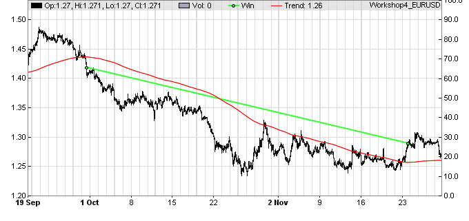 The black jagged line in the chart above is the raw price curve, the red line is the filtered curve. You can see that it lags behind the black curve a little, which is typical of smoothing indicators. It has a peak at the end of September and thus entered a short trade (tiny green dot). The red line continues going down all the way until November 23, when a valley was reached. A long trade (not shown in this chart) was then entered and the short trade was closed by reversal (other tiny green dot). The green straight line connects the entry and exit points of the trade. It was open almost 2 months and made in that time a profit of ~ 13 cents per unit, or 1300 pips.
The only remaining question is – which indicator shall we use for filtering out the high frequencies, the ripples and jaggies, from the price curve? We’re spoilt for choice.
The Smoothing Candidates
Smoothing a curve in some way is a common task of all trend strategies. Consequently, there’s a multitude of smoothing, averaging, low-lag and spectral filter indicators at our disposal. We have to test them. The following candidates were selected for the experiment, traditional indicators as well as fancier algorithms:
- SMA, the simple moving average, the sum of the last n prices divided by n.
- EMA, exponential moving average, the current price multiplied with a small factor plus the last EMA multiplied with a large factor. The sum of both factors must be 1. This is a first order lowpass filter.
- LowPass, a second order lowpass filter with the following source code:
var LowPass(var *Data,int Period) { var* LP = series(Data[0]); var a = 2.0/(1+Period); return LP[0] = (a-0.25*a*a)*Data[0] + 0.5*a*a*Data[1] - (a-0.75*a*a)*Data[2] + 2*(1.-a)*LP[1] - (1.-a)*(1.-a)*LP[2]; } - HMA, the Hull Moving Average, with the following source code:
var HMA(var *Data,int Period) { return WMA(series(2*WMA(Data,Period/2)-WMA(Data,Period),sqrt(Period)) } - ZMA, Ehler’s Zero-Lag Moving Average, an EMA with a correction term for removing lag. This is the source code:
var ZMA(var *Data,int Period) { var *ZMA = series(Data[0]); var a = 2.0/(1+Period); var Ema = EMA(Data,Period); var Error = 1000000; var Gain, GainLimit=5, BestGain=0; for(Gain = -GainLimit; Gain < GainLimit; Gain += 0.1) { ZMA[0] = a*(Ema + Gain*(Data[0]-ZMA[1])) + (1-a)*ZMA[1]; var NewError = Data[0] - ZMA[0]; if(abs(Error) < newError) { Error = abs(newError); BestGain = Gain; } } return ZMA[0] = a*(Ema + BestGain*(Data[0]-ZMA[1])) + (1-a)*ZMA[1]; } - ALMA, Arnaud Legoux Moving Average, based on a shifted Gaussian distribution (described in this paper):
var ALMA(var *Data, int Period) { var m = floor(0.85*(Period-1)); var s = Period/6.0; var alma = 0., wSum = 0.; int i; for (i = 0; i < Period; i++) { var w = exp(-(i-m)*(i-m)/(2*s*s)); alma += Data[Period-1-i] * w; wSum += w; } return alma / wSum; } - Laguerre, a 4-element Laguerre filter:
var Laguerre(var *Data, var alpha) { var *L = series(Data[0]); L[0] = alpha*Data[0] + (1-alpha)*L[1]; L[2] = -(1-alpha)*L[0] + L[1] + (1-alpha)*L[2+1]; L[4] = -(1-alpha)*L[2] + L[2+1] + (1-alpha)*L[4+1]; L[6] = -(1-alpha)*L[4] + L[4+1] + (1-alpha)*L[6+1]; return (L[0]+2*L[2]+2*L[4]+L[6])/6; } - Linear regression, fits a straight line between the data points in a way that the distance between each data point and the line is minimized by the least-squares rule.
- Smooth, John Ehlers’ “Super Smoother”, a 2-pole Butterworth filter combined with a 2-bar SMA that suppresses the Nyquist frequency:
var Smooth(var *Data,int Period) { var f = (1.414*PI) / Period; var a = exp(-f); var c2 = 2*a*cos(f); var c3 = -a*a; var c1 = 1 - c2 - c3; var *S = series(Data[0]); return S[0] = c1*(Data[0]+Data[1])*0.5 + c2*S[1] + c3*S[2]; } - Decycle, another low-lag indicator by John Ehlers. His decycler is simply the difference between the price and its fluctuation, retrieved with a highpass filter:
var Decycle(var* Data,int Period)
{
  return Data[0]-HighPass2(Data,Period);
}
The above source codes have been taken from the indicators.c file of the Zorro platform, which contains source codes of all supplied indicators.
Comparing Step Responses
What is the best of all those indicators? For a first impression here’s a chart showing them reacting on a simulated sudden price step. You can see that some react slow, some very slow, some fast, and some overshoot: 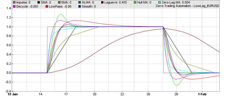 You can generate such a step response diagram with this Zorro script:
// compare the step responses of some low-lag MAs
function run()
{
  set(PLOTNOW);
  BarPeriod = 60;
  MaxBars = 1000;
  LookBack = 150;
  asset("");   // don't load an asset
  ColorUp = ColorDn = 0;  // don't plot a price curve
  PlotWidth = 800;
  PlotHeight1 = 400;

  var *Impulse = series(ifelse(Bar>200 && Bar<400,1,0)); // 0->1 impulse
  int Period = 50;
  plot("Impulse",Impulse[0],0,GREY);
  plot("SMA",SMA(Impulse,Period),0,BLACK);
  plot("EMA",EMA(Impulse,Period),0,0x808000);
  plot("ALMA",ALMA(Impulse,Period),0,0x008000);
  plot("Laguerre",Laguerre(Impulse,4.0/Period),0,0x800000);
  plot("Hull MA",HMA(Impulse,Period),0,0x00FF00);
  plot("Zero-Lag MA",ZMA(Impulse,Period),0,0x00FFFF);
  plot("Decycle",Decycle(Impulse,Period),0,0xFF00FF);
  plot("LowPass",LowPass(Impulse,Period),0,0xFF0000);
  plot("Smooth",Smooth(Impulse,Period),0,0x0000FF);
}
We can see that from all the indicators, the ALMA seems to be the best representation of the step, while the ZMA produces the fastest response with no overshoot, the Decycler the fastest with some overshoot, and Laguerre lags a lot behind anything else. Obviously, all this has not much meaning because the time period parameters of the indicators are not really comparable. So the step response per se does not reveal if the indicator is well suited for trend detection. We have no choice: We must use them all.
The Trend Experiment
For the experiment, all smoothing indicators above will be applied to a currency, a stock index, and a commodity, and will compete in exploiting trend. Because different time frames can represent different trader groups and thus different markets, the indicators will be applied to price curves made of 15-minutes, 1-hour, and 4-hours bars. And we’ll also try different indicator time periods in 10 steps from 10 to 10000 bars.
So we’ll have to program 10 indicators * 3 assets * 3 bar sizes * 10 time periods = 900 systems. Some of the 900 results will be positive, some negative, and some zero. If there are no significant positive results, we’ll have to conclude that trend in price curves either does not exist, or can at least not be exploited with this all-too-obvious method. However we’ll likely get some winning systems, if only for statistical reasons.
The next step will be checking if their profits are for real or just caused by a statistical effect dubbed Data Mining Bias. There is a method to measure Data Mining Bias from the resulting equity curves: the notorious White’s Reality Check. We’ll apply that check to the results of our experiment. If some systems survive White’s Reality Check, we’ll have the once-and-for-all proof that markets are ineffective, trends really exist, and algorithmic trend trading works.
Congratulations to this new page jcl. You allways adress very interesting items. I’m following your Zorro User Community platform already very seriosly and some of your comments at other trade forums and by this I’m wondering where you get all the time from to support so many forums and blogs. Please give some informations how you differ content of Zorro and this Financial Hackers page in future. What is the main idea of this page compared to orig. Zorro page. Thanks a lot for your replay.
Thanks for the kind words. The main purpose is publishing the results of our trade system research and experiments. So far, when results did not end up in some Zorro system, they were discarded. But some results were interesting and besides, one learns from failures much more than from success. Thus I’m going to publish some of the experiences and experiments on this blog in regular intervals.
Hi,
I noticed in the return statement for the Lowpass code LP[1] and LP[2] are used in addition to Data[1] and Data[2]. But if var* LP = series(Data[0]) copies the values from Data into LP, aren’t LP[1] and LP[2] just the same as Data[1] and Data[2] (the same thing happens in Smooth)? I tested this out in Zorro by plotting a lowpass filtered price series and got different results when I switched out LP[1] and LP[2] with Data[1] and Data[2], but I don’t understand why. Something to do with series?
No, they are not the same. LP[1] is just the previous value of LP[0]. Data[0] is only used for initially filling the series with the current price when it is created. Otherwise, LP[1] and LP[2] were 0 at the beginning.
I’m a fully systematic futures trader and this is a truly superb blog, with many fascinating ideas which will spike further research in serious traders. You ought to be proud of stimulating this kind of discussion, kudos to you Sir.
Just wondering if this Zorro MA can be transferred into excel
You are awesome! After seeing these lots of typical trial and error TA tutorials, I finally find some place where contains real things.
Thanks, nice overview.
However there are some small definition typos in your post.
In the paragraph ‘Comparing Impulse Responses’ it would be advisable to rename the text ‘impulse response’ to ‘unit step response’ or more simply ‘step response’.
An ‘impulse response’ is a reaction to a spike (impulse) of a certain amplitude.
An ‘unit impulse response’ is a reaction to a spike of amplitude 1.0.
A ‘step response’ is a reaction to a step,
An ‘unit step response’ is a reaction to a step of amplitude 1.0
You’re right, it’s a step response, not an impulse response.
Based on your article, I was using a lot the ALMA … until i noticed that it is almost equivalent to an SMA of lower period !
Just compare SMA 9 and ALMA 22, SMA 20 and ALMA 51, SMA 50 and ALMA 125… You will have the same thing, with no clear advantages to the ALMA.
Hmm, maybe its just me but SMA and Alma with these periods look clearly different to me.
Excellent. Thanks for sharing trend indicators. Functions like below that you shared are very useful to learn about how the indicators work internally
var Laguerre(var *Data, var alpha)
{
var *L = series(Data[0]);
L[0] = alpha*Data[0] + (1-alpha)*L[1];
L[2] = -(1-alpha)*L[0] + L[1] + (1-alpha)*L[2+1];
L[4] = -(1-alpha)*L[2] + L[2+1] + (1-alpha)*L[4+1];
L[6] = -(1-alpha)*L[4] + L[4+1] + (1-alpha)*L[6+1];
return (L[0]+2*L[2]+2*L[4]+L[6])/6;
}
Can you also please share the logic for BandPass filter similarly?
I tried all these trend indicators namely SuperSmoother, Laguerre, ALMA, LowPass filters into a ML model.
The AUCs/predictability of these features is not great
SuperSmoother 0.5257
Laguerre 0.53006
Decycle: 0.5322
alma: 0.5
The predictive power of these features in ML models is comparable to FMA which was 0.529 and to EMA which is 0.526. These do not offer any upside in predictability of returns