
It’s time for the 5th and final part of the Build Better Strategies series. In part 3 we’ve discussed the development process of a model-based system, and consequently we’ll conclude the series with developing a data-mining system. The principles of data mining and machine learning have been the topic of part 4. For our short-term trading example we’ll use a deep learning algorithm, a stacked autoencoder, but it will work in the same way with many other machine learning algorithms. With today’s software tools, only about 20 lines of code are needed for a machine learning strategy. I’ll try to explain all steps in detail.
Our example will be a research project – a machine learning experiment for answering two questions. Does a more complex algorithm – such as, more neurons and deeper learning – produce a better prediction? And are short-term price moves predictable by short-term price history? The last question came up due to my scepticism about price action trading in the previous part of this series. I got several emails asking about the “trading system generators” or similar price action tools that are praised on some websites. There is no hard evidence that such tools ever produced any profit (except for their vendors) – but does this mean that they all are garbage? We’ll see.
Our experiment is simple: We collect information from the last candles of a price curve, feed it in a deep learning neural net, and use it to predict the next candles. My hypothesis is that a few candles don’t contain any useful predictive information. Of course, a nonpredictive outcome of the experiment won’t mean that I’m right, since I could have used wrong parameters or prepared the data badly. But a predictive outcome would be a hint that I’m wrong and price action trading can indeed be profitable.
Machine learning strategy development
Step 1: The target variable
To recap the previous part: a supervised learning algorithm is trained with a set of features in order to predict a target variable. So the first thing to determine is what this target variable shall be. A popular target, used in most papers, is the sign of the price return at the next bar. Better suited for prediction, since less susceptible to randomness, is the price difference to a more distant prediction horizon, like 3 bars from now, or same day next week. Like almost anything in trading systems, the prediction horizon is a compromise between the effects of randomness (less bars are worse) and predictability (less bars are better).
Sometimes you’re not interested in directly predicting price, but in predicting some other parameter – such as the current leg of a Zigzag indicator – that could otherwise only be determined in hindsight. Or you want to know if a certain market inefficiency will be present in the next time, especially when you’re using machine learning not directly for trading, but for filtering trades in a model-based system. Or you want to predict something entirely different, for instance the probability of a market crash tomorrow. All this is often easier to predict than the popular tomorrow’s return.
In our price action experiment we’ll use the return of a short-term price action trade as target variable. Once the target is determined, next step is selecting the features.
Step 2: The features
A price curve is the worst case for any machine learning algorithm. Not only does it carry little signal and mostly noise, it is also nonstationary and the signal/noise ratio changes all the time. The exact ratio of signal and noise depends on what is meant with “signal”, but it is normally too low for any known machine learning algorithm to produce anything useful. So we must derive features from the price curve that contain more signal and less noise. Signal, in that context, is any information that can be used to predict the target, whatever it is. All the rest is noise.
Thus, selecting the features is critical for success – even more critical than deciding which machine learning algorithm you’re going to use. There are two approaches for selecting features. The first and most common is extracting as much information from the price curve as possible. Since you do not know where the information is hidden, you just generate a wild collection of indicators with a wide range of parameters, and hope that at least a few of them will contain the information that the algorithm needs. This is the approach that you normally find in the literature. The problem of this method: Any machine learning algorithm is easily confused by nonpredictive predictors. So it won’t do to just throw 150 indicators at it. You need some preselection algorithm that determines which of them carry useful information and which can be omitted. Without reducing the features this way to maybe eight or ten, even the deepest learning algorithm won’t produce anything useful.
The other approach, normally for experiments and research, is using only limited information from the price curve. This is the case here: Since we want to examine price action trading, we only use the last few prices as inputs, and must discard all the rest of the curve. This has the advantage that we don’t need any preselection algorithm since the number of features is limited anyway. Here are the two simple predictor functions that we use in our experiment (in C):
var change(int n)
{
	return scale((priceClose(0) - priceClose(n))/priceClose(0),100)/100;
}

var range(int n)
{
	return scale((HH(n) - LL(n))/priceClose(0),100)/100;
}
The two functions are supposed to carry the necessary information for price action: per-bar movement and volatility. The change function is the difference of the current price to the price of n bars before, divided by the current price. The range function is the total high-low distance of the last n candles, also in divided by the current price. And the scale function centers and compresses the values to the +/-100 range, so we divide them by 100 for getting them normalized to +/-1. We remember that normalizing is needed for machine learning algorithms.
Step 3: Preselecting predictors
When you have selected a large number of indicators or other signals as features for your algorithm, you must determine which of them is useful and which not. There are many methods for reducing the number of features, for instance:
- Determine the correlations between the signals. Remove those with a strong correlation to other signals, since they do not contribute to the information.
- Compare the information content of signals directly, with algorithms like information entropy or decision trees.
- Determine the information content indirectly by comparing the signals with randomized signals; there are some software libraries for this, such as the R Boruta package.
- Use an algorithm like Principal Components Analysis (PCA) for generating a new signal set with reduced dimensionality.
- Use genetic optimization for determining the most important signals just by the most profitable results from the prediction process. Great for curve fitting if you want to publish impressive results in a research paper.
Reducing the number of features is important for most machine learning algorithms, including shallow neural nets. For deep learning it’s less important, since deep nets with many neurons are normally able to process huge feature sets and discard redundant features. For our experiment we do not preselect or preprocess the features, but you can find useful information about this in articles (1), (2), and (3) listed at the end of the page.
Step 4: Select the machine learning algorithm
R offers many different ML packages, and any of them offers many different algorithms with many different parameters. Even if you already decided about the method – here, deep learning – you have still the choice among different approaches and different R packages. Most are quite new, and you can find not many empirical information that helps your decision. You have to try them all and gain experience with different methods. For our experiment we’ve choosen the Deepnet package, which is probably the simplest and easiest to use deep learning library. This keeps our code short. We’re using its Stacked Autoencoder (SAE) algorithm for pre-training the network. Deepnet also offers a Restricted Boltzmann Machine (RBM) for pre-training, but I could not get good results from it. There are other and more complex deep learning packages for R, so you can spend a lot of time checking out all of them.
How pre-training works is easily explained, but why it works is a different matter. As to my knowledge, no one has yet come up with a solid mathematical proof that it works at all. Anyway, imagine a large neural net with many hidden layers:
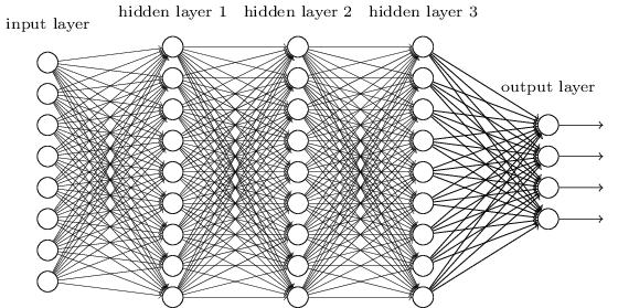
Training the net means setting up the connection weights between the neurons. The usual method is error backpropagation. But it turns out that the more hidden layers you have, the worse it works. The backpropagated error terms get smaller and smaller from layer to layer, causing the first layers of the net to learn almost nothing. Which means that the predicted result becomes more and more dependent of the random initial state of the weights. This severely limited the complexity of layer-based neural nets and therefore the tasks that they can solve. At least until 10 years ago.
In 2006 scientists in Toronto first published the idea to pre-train the weights with an unsupervised learning algorithm, a restricted Boltzmann machine. This turned out a revolutionary concept. It boosted the development of artificial intelligence and allowed all sorts of new applications from Go-playing machines to self-driving cars. Meanwhile, several new improvements and algorithms for deep learning have been found. A stacked autoencoder works this way:
- Select the hidden layer to train; begin with the first hidden layer. Connect its outputs to a temporary output layer that has the same structure as the network’s input layer.
- Feed the network with the training samples, but without the targets. Train it so that the first hidden layer reproduces the input signal – the features – at its outputs as exactly as possible. The rest of the network is ignored. During training, apply a ‘weight penalty term’ so that as few connection weights as possible are used for reproducing the signal.
- Now feed the outputs of the trained hidden layer to the inputs of the next untrained hidden layer, and repeat the training process so that the input signal is now reproduced at the outputs of the next layer.
- Repeat this process until all hidden layers are trained. We have now a ‘sparse network’ with very few layer connections that can reproduce the input signals.
- Now train the network with backpropagation for learning the target variable, using the pre-trained weights of the hidden layers as a starting point.
The hope is that the unsupervised pre-training process produces an internal noise-reduced abstraction of the input signals that can then be used for easier learning the target. And this indeed appears to work. No one really knows why, but several theories – see paper (4) below – try to explain that phenomenon.
Step 5: Generate a test data set
We first need to produce a data set with features and targets so that we can test our prediction process and try out parameters. The features must be based on the same price data as in live trading, and for the target we must simulate a short-term trade. So it makes sense to generate the data not with R, but with our trading platform, which is anyway a lot faster. Here’s a small Zorro script for this, DeepSignals.c:
function run()
{
	StartDate = 20140601; // start two years ago
	BarPeriod = 60; // use 1-hour bars
	LookBack = 100; // needed for scale()

	set(RULES);   // generate signals
	LifeTime = 3; // prediction horizon
	Spread = RollLong = RollShort = Commission = Slippage = 0;

	adviseLong(SIGNALS+BALANCED,0,
		change(1),change(2),change(3),change(4),
		range(1),range(2),range(3),range(4));
	enterLong();
}
We’re generating 2 years of data with features calculated by our above defined change and range functions. Our target is the result of a trade with 3 bars life time. Trading costs are set to zero, so in this case the result is equivalent to the sign of the price difference at 3 bars in the future. The adviseLong function is described in the Zorro manual; it is a mighty function that automatically handles training and predicting and allows to use any R-based machine learning algorithm just as if it were a simple indicator.
In our code, the function uses the next trade return as target, and the price changes and ranges of the last 4 bars as features. The SIGNALS flag tells it not to train the data, but to export it to a .csv file. The BALANCED flag makes sure that we get as many positive as negative returns; this is important for most machine learning algorithms. Run the script in [Train] mode with our usual test asset EUR/USD selected. It generates a spreadsheet file named DeepSignalsEURUSD_L.csv that contains the features in the first 8 columns, and the trade return in the last column.
Step 6: Calibrate the algorithm
Complex machine learning algorithms have many parameters to adjust. Some of them offer great opportunities to curve-fit the algorithm for publications. Still, we must calibrate parameters since the algorithm rarely works well with its default settings. For this, here’s an R script that reads the previously created data set and processes it with the deep learning algorithm (DeepSignal.r):
library('deepnet', quietly = T)
library('caret', quietly = T)

neural.train = function(model,XY)
{
  XY <- as.matrix(XY)
  X <- XY[,-ncol(XY)]
  Y <- XY[,ncol(XY)]
  Y <- ifelse(Y > 0,1,0)
  Models[[model]] <<- sae.dnn.train(X,Y,
      hidden = c(50,100,50),
      activationfun = "tanh",
      learningrate = 0.5,
      momentum = 0.5,
      learningrate_scale = 1.0,
      output = "sigm",
      sae_output = "linear",
      numepochs = 100,
      batchsize = 100,
      hidden_dropout = 0,
      visible_dropout = 0)
}

neural.predict = function(model,X)
{
  if(is.vector(X)) X <- t(X)
  return(nn.predict(Models[[model]],X))
}

neural.init = function()
{
  set.seed(365)
  Models <<- vector("list")
}

TestOOS = function()
{
  neural.init()
  XY <<- read.csv('C:/Zorro/Data/DeepSignalsEURUSD_L.csv',header = F)
  splits <- nrow(XY)*0.8
  XY.tr <<- head(XY,splits);
  XY.ts <<- tail(XY,-splits)
  neural.train(1,XY.tr)
  X <<- XY.ts[,-ncol(XY.ts)]
  Y <<- XY.ts[,ncol(XY.ts)]
  Y.ob <<- ifelse(Y > 0,1,0)
  Y <<- neural.predict(1,X)
  Y.pr <<- ifelse(Y > 0.5,1,0)
  confusionMatrix(Y.pr,Y.ob)
}
We’ve defined three functions neural.train, neural.predict, and neural.init for training, predicting, and initializing the neural net. The function names are not arbitrary, but follow the convention used by Zorro’s advise(NEURAL,..) function. It doesn’t matter now, but will matter later when we use the same R script for training and trading the deep learning strategy. A fourth function, TestOOS, is used for out-of-sample testing our setup.
The function neural.init seeds the R random generator with a fixed value (365 is my personal lucky number). Otherwise we would get a slightly different result any time, since the neural net is initialized with random weights. It also creates a global R list named “Models”. Most R variable types don’t need to be created beforehand, some do (don’t ask me why). The ‘<<-‘ operator is for accessing a global variable from within a function.
The function neural.train takes as input a model number and the data set to be trained. The model number identifies the trained model in the “Models” list. A list is not really needed for this test, but we’ll need it for more complex strategies that train more than one model. The matrix containing the features and target is passed to the function as second parameter. If the XY data is not a proper matrix, which frequently happens in R depending on how you generated it, it is converted to one. Then it is split into the features (X) and the target (Y), and finally the target is converted to 1 for a positive trade outcome and 0 for a negative outcome.
The network parameters are then set up. Some are obvious, others are free to play around with:
- The network structure is given by the hidden vector: c(50,100,50) defines 3 hidden layers, the first with 50, second with 100, and third with 50 neurons. That’s the parameter that we’ll later modify for determining whether deeper is better.
- The activation function converts the sum of neuron input values to the neuron output; most often used are sigmoid that saturates to 0 or 1, or tanh that saturates to -1 or +1.
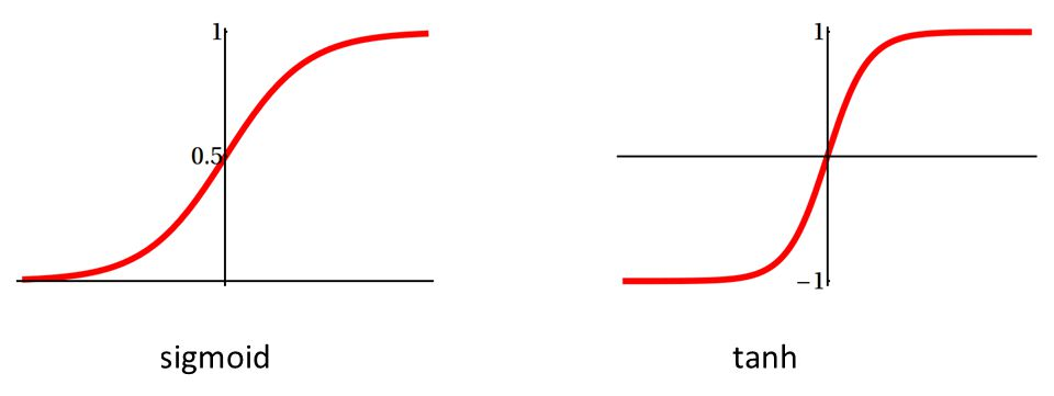
We use tanh here since our signals are also in the +/-1 range. The output of the network is a sigmoid function since we want a prediction in the 0..1 range. But the SAE output must be “linear” so that the Stacked Autoencoder can reproduce the analog input signals on the outputs. Recently in fashion came RLUs, Rectified Linear Units, as activation functions for internal layers. RLUs are faster and partially overcome the above mentioned backpropagation problem, but are not supported by deepnet.
- The learning rate controls the step size for the gradient descent in training; a lower rate means finer steps and possibly more precise prediction, but longer training time.
- Momentum adds a fraction of the previous step to the current one. It prevents the gradient descent from getting stuck at a tiny local minimum or saddle point.
- The learning rate scale is a multiplication factor for changing the learning rate after each iteration (I am not sure for what this is good, but there may be tasks where a lower learning rate on higher epochs improves the training).
- An epoch is a training iteration over the entire data set. Training will stop once the number of epochs is reached. More epochs mean better prediction, but longer training.
- The batch size is a number of random samples – a mini batch – taken out of the data set for a single training run. Splitting the data into mini batches speeds up training since the weight gradient is then calculated from fewer samples. The higher the batch size, the better is the training, but the more time it will take.
- The dropout is a number of randomly selected neurons that are disabled during a mini batch. This way the net learns only with a part of its neurons. This seems a strange idea, but can effectively reduce overfitting.
All these parameters are common for neural networks. Play around with them and check their effect on the result and the training time. Properly calibrating a neural net is not trivial and might be the topic of another article. The parameters are stored in the model together with the matrix of trained connection weights. So they need not to be given again in the prediction function, neural.predict. It takes the model and a vector X of features, runs it through the layers, and returns the network output, the predicted target Y. Compared with training, prediction is pretty fast since it only needs a couple thousand multiplications. If X was a row vector, it is transposed and this way converted to a column vector, otherwise the nn.predict function won’t accept it.
Use RStudio or some similar environment for conveniently working with R. Edit the path to the .csv data in the file above, source it, install the required R packages (deepnet, e1071, and caret), then call the TestOOS function from the command line. If everything works, it should print something like that:
> TestOOS()
begin to train sae ......
training layer 1 autoencoder ...
####loss on step 10000 is : 0.000079
training layer 2 autoencoder ...
####loss on step 10000 is : 0.000085
training layer 3 autoencoder ...
####loss on step 10000 is : 0.000113
sae has been trained.
begin to train deep nn ......
####loss on step 10000 is : 0.123806
deep nn has been trained.
Confusion Matrix and Statistics

          Reference
Prediction    0    1
         0 1231  808
         1  512  934

               Accuracy : 0.6212
                 95% CI : (0.6049, 0.6374)
    No Information Rate : 0.5001
    P-Value [Acc > NIR] : < 2.2e-16

                  Kappa : 0.2424
 Mcnemar's Test P-Value : 4.677e-16

            Sensitivity : 0.7063
            Specificity : 0.5362
         Pos Pred Value : 0.6037
         Neg Pred Value : 0.6459
             Prevalence : 0.5001
         Detection Rate : 0.3532
   Detection Prevalence : 0.5851
      Balanced Accuracy : 0.6212

       'Positive' Class : 0

>
TestOOS reads first our data set from Zorro’s Data folder. It splits the data in 80% for training (XY.tr) and 20% for out-of-sample testing (XY.ts). The training set is trained and the result stored in the Models list at index 1. The test set is further split in features (X) and targets (Y). Y is converted to binary 0 or 1 and stored in Y.ob, our vector of observed targets. We then predict the targets from the test set, convert them again to binary 0 or 1 and store them in Y.pr. For comparing the observation with the prediction, we use the confusionMatrix function from the caret package.
A confusion matrix of a binary classifier is simply a 2×2 matrix that tells how many 0’s and how many 1’s had been predicted wrongly and correctly. A lot of metrics are derived from the matrix and printed in the lines above. The most important at the moment is the 62% prediction accuracy. This may hint that I bashed price action trading a little prematurely. But of course the 62% might have been just luck. We’ll see that later when we run a WFO test.
A final advice: R packages are occasionally updated, with the possible consequence that previous R code suddenly might work differently, or not at all. This really happens, so test carefully after any update.
Step 7: The strategy
Now that we’ve tested our algorithm and got some prediction accuracy above 50% with a test data set, we can finally code our machine learning strategy. In fact we’ve already coded most of it, we just must add a few lines to the above Zorro script that exported the data set. This is the final script for training, testing, and (theoretically) trading the system (DeepLearn.c):
#include <r.h>

function run()
{
	StartDate = 20140601;
	BarPeriod = 60;	// 1 hour
	LookBack = 100;

	WFOPeriod = 252*24; // 1 year
	DataSplit = 90;
	NumCores = -1;  // use all CPU cores but one

	set(RULES);
	Spread = RollLong = RollShort = Commission = Slippage = 0;
	LifeTime = 3;
	if(Train) Hedge = 2;

	if(adviseLong(NEURAL+BALANCED,0,
		change(1),change(2),change(3),change(4),
		range(1),range(2),range(3),range(4)) > 0.5)
		enterLong();
	if(adviseShort() > 0.5)
		enterShort();
}
We’re using a WFO cycle of one year, split in a 90% training and a 10% out-of-sample test period. You might ask why I have earlier used two year’s data and a different split, 80/20, for calibrating the network in step 5. This is for using differently composed data for calibrating and for walk forward testing. If we used exactly the same data, the calibration might overfit it and compromise the test.
The selected WFO parameters mean that the system is trained with about 225 days data, followed by a 25 days test or trade period. Thus, in live trading the system would retrain every 25 days, using the prices from the previous 225 days. In the literature you’ll sometimes find the recommendation to retrain a machine learning system after any trade, or at least any day. But this does not make much sense to me. When you used almost 1 year’s data for training a system, it can obviously not deteriorate after a single day. Or if it did, and only produced positive test results with daily retraining, I would strongly suspect that the results are artifacts by some coding mistake.
Training a deep network takes really a long time, in our case about 10 minutes for a network with 3 hidden layers and 200 neurons. In live trading this would be done by a second Zorro process that is automatically started by the trading Zorro. In the backtest, the system trains at any WFO cycle. Therefore using multiple cores is recommended for training many cycles in parallel. The NumCores variable at -1 activates all CPU cores but one. Multiple cores are only available in Zorro S, so a complete walk forward test with all WFO cycles can take several hours with the free version.
In the script we now train both long and short trades. For this we have to allow hedging in Training mode, since long and short positions are open at the same time. Entering a position is now dependent on the return value from the advise function, which in turn calls either the neural.train or the neural.predict function from the R script. So we’re here entering positions when the neural net predicts a result above 0.5.
The R script is now controlled by the Zorro script (for this it must have the same name, DeepLearn.r, only with different extension). It is identical to our R script above since we’re using the same network parameters. Only one additional function is needed for supporting a WFO test:
neural.save = function(name)
{
  save(Models,file=name)
}
The neural.save function stores the Models list – it now contains 2 models for long and for short trades – after every training run in Zorro’s Data folder. Since the models are stored for later use, we do not need to train them again for repeated test runs.
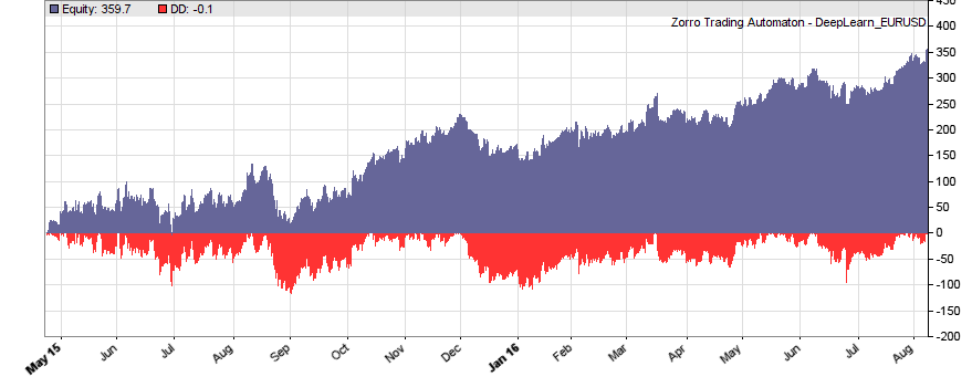
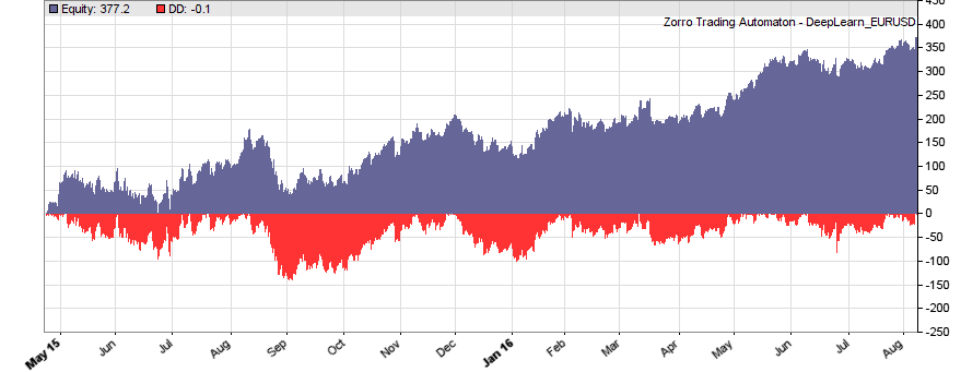
This is the WFO equity curve generated with the script above (EUR/USD, without trading costs):
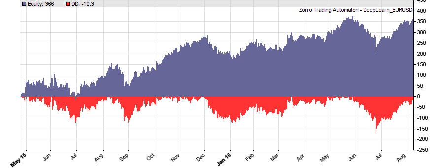
Although not all WFO cycles get a positive result, it seems that there is some predictive effect. The curve is equivalent to an annual return of 89%, achieved with a 50-100-50 hidden layer structure. We’ll check in the next step how different network structures affect the result.
Since the neural.init, neural.train, neural.predict, and neural.save functions are automatically called by Zorro’s adviseLong/adviseShort functions, there are no R functions directly called in the Zorro script. Thus the script can remain unchanged when using a different machine learning method. Only the DeepLearn.r script must be modified and the neural net, for instance, replaced by a support vector machine. For trading such a machine learning system live on a VPS, make sure that R is also installed on the VPS, the needed R packages are installed, and the path to the R terminal set up in Zorro’s ini file. Otherwise you’ll get an error message when starting the strategy.
Step 8: The experiment
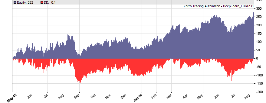
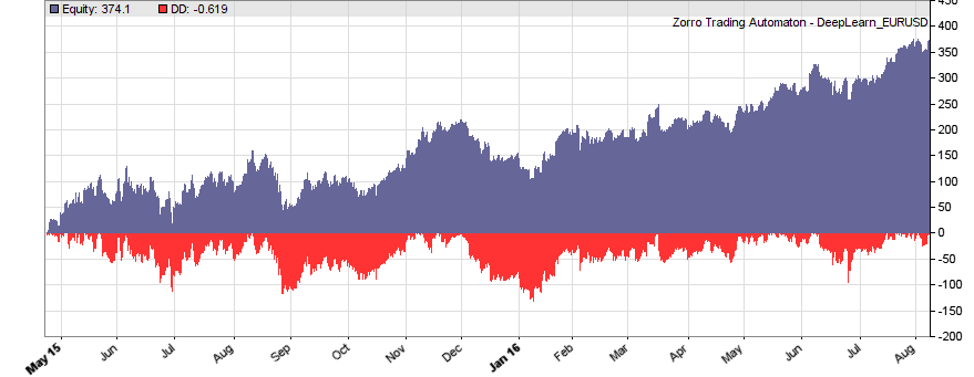
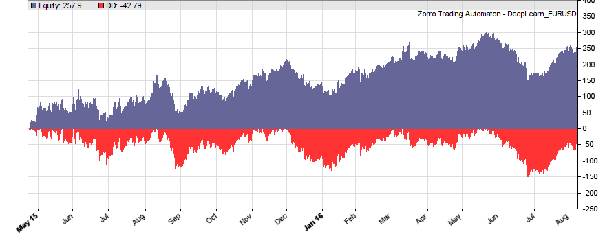
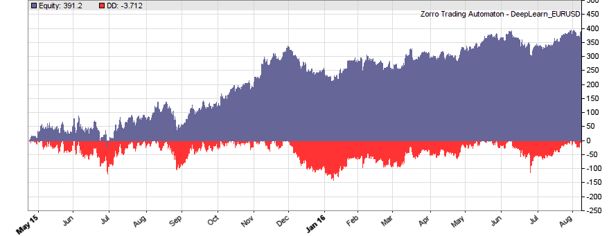
If our goal had been developing a strategy, the next steps would be the reality check, risk and money management, and preparing for live trading just as described under model-based strategy development. But for our experiment we’ll now run a series of tests, with the number of neurons per layer increased from 10 to 100 in 3 steps, and 1, 2, or 3 hidden layers (deepnet does not support more than 3). So we’re looking into the following 9 network structures: c(10), c(10,10), c(10,10,10), c(30), c(30,30), c(30,30,30), c(100), c(100,100), c(100,100,100). For this experiment you need an afternoon even with a fast PC and in multiple core mode. Here are the results (SR = Sharpe ratio, R2 = slope linearity):
| * 10 neurons | * 30 neurons | * 100 neurons | |
| 1 |
 |
 |
 |
| 2 |
 |
 |
 |
| 3 |
 |
 |
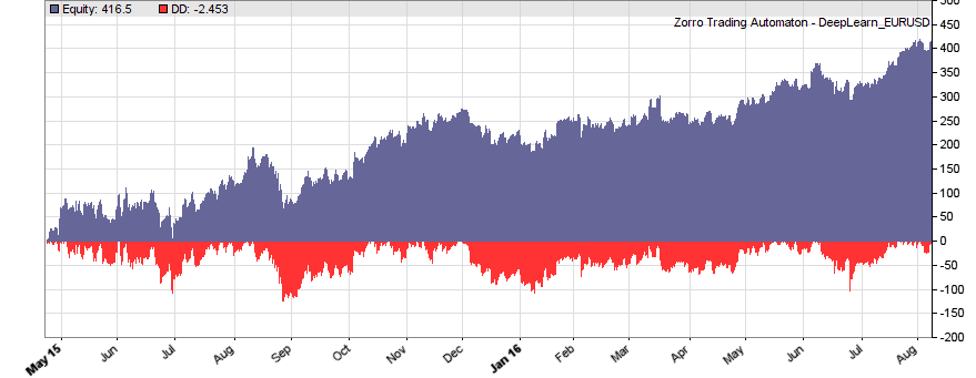 |
We see that a simple net with only 10 neurons in a single hidden layer won’t work well for short-term prediction. Network complexity clearly improves the performance, however only up to a certain point. A good result for our system is already achieved with 3 layers x 30 neurons. Even more neurons won’t help much and sometimes even produce a worse result. This is no real surprise, since for processing only 8 inputs, 300 neurons can likely not do a better job than 100.
Conclusion
Our goal was determining if a few candles can have predictive power and how the results are affected by the complexity of the algorithm. The results seem to suggest that short-term price movements can indeed be predicted sometimes by analyzing the changes and ranges of the last 4 candles. The prediction is not very accurate – it’s in the 58%..60% range, and most systems of the test series become unprofitable when trading costs are included. Still, I have to reconsider my opinion about price action trading. The fact that the prediction improves with network complexity is an especially convincing argument for short-term price predictability.
It would be interesting to look into the long-term stability of predictive price patterns. For this we had to run another series of experiments and modify the training period (WFOPeriod in the script above) and the 90% IS/OOS split. This takes longer time since we must use more historical data. I have done a few tests and found so far that a year seems to be indeed a good training period. The system deteriorates with periods longer than a few years. Predictive price patterns, at least of EUR/USD, have a limited lifetime.
Where can we go from here? There’s a plethora of possibilities, for instance:
- Use inputs from more candles and process them with far bigger networks with thousands of neurons.
- Use oversampling for expanding the training data. Prediction always improves with more training samples.
- Compress time series f.i. with spectal analysis and analyze not the candles, but their frequency representation with machine learning methods.
- Use inputs from many candles – such as, 100 – and pre-process adjacent candles with one-dimensional convolutional network layers.
- Use recurrent networks. Especially LSTM could be very interesting for analyzing time series – and as to my knowledge, they have been rarely used for financial prediction so far.
- Use an ensemble of neural networks for prediction, such as Aronson’s “oracles” and “comitees”.
Papers / Articles
(1) A.S.Sisodiya, Reducing Dimensionality of Data
(2) K.Longmore, Machine Learning for Financial Prediction
(3) V.Perervenko, Selection of Variables for Machine Learning
(4) D.Erhan et al, Why Does Pre-training Help Deep Learning?
I’ve added the C and R scripts to the 2016 script repository. You need both in Zorro’s Strategy folder. Zorro version 1.474, and R version 3.2.5 (64 bit) was used for the experiment, but it should also work with other versions.
Excellent post!
I’ve tested your strategy using 30min AAPL data but “sae.dnn.train” returns all NaN in training.
(It works just decreasing neurons to less than (5,10,5)… but accuracy is 49%)
Can you help me to understand why?
Thanks in advance
If you have not changed any SAE parameters, look into the .csv data. It is then the only difference to the EUR/USD test. Maybe something is wrong with it.
Another fantastic article, jcl. Zorro is a remarkable environment for these experiments. Thanks for sharing your code and your approach – this really opens up an incredible number of possibilities to anyone willing to invest the time to learn how to use Zorro.
The problem with AAPL 30min data was related to the normalizing method I used (X-mean/SD).
The features range was not between -1:1 and I assume that sae.dnn need it to work…
Anyway performances are not comparable to yours 🙂
Thanks
Hi,
Great article!
I have one question:
why do you use Zorro for creating the features in the csv file and then opening it in R?
why not create the file with all the features in R in a few lines and do the training on the file when you are already in R? instead of getting inside Zorro and then to R.
When you want R to create the features, you must still transmit the price data and the targets from Zorro to R. So you are not gaining much. Creating the features in Zorro results usually in shorter code and faster training. Features in R make only sense when you need some R package for calculating them.
Really helpful and interesting article! I would like to know if there are any English version of the book:
“Das Börsenhackerbuch: Finanziell unabhängig durch algorithmische Handelssysteme”
I am really interested on it,
Thanks!
Not yet, but an English version is planned.
Thanks JCL! Please let me now when the English version is ready, because I am really interested on it.
Thanks a lot!
Works superbly (as always). Many thanks. One small note, if you have the package “dlm” loaded in R, TestOOS will fail with error: “Error in TestOOS() : cannot change value of locked binding for ‘X'”. This is due to there being a function X in the dlm package, so the name is locked when the package is loaded. Easily fixed by either renaming occurrences of the variable X to something else, or temporarily detaching the dlm package with: detach(“package:dlm”, unload=TRUE)
Thanks for the info with the dlm package. I admit that ‘X’ is not a particular good name for a variable, but a function named ‘X’ in a distributed package is even a bit worse.
I would agree… 🙂
Results below were generated by revised version of DeepSignals.r – only change was use of LSTM net from the rnn package on CRAN. The authors of the package regard their LSTM implementation as “experimental” and do not feel it is as yet learning properly, so hopefully more improvement to come there. (Spent ages trying to accomplish the LSTM element using the mxnet package but gave up as couldn’t figure out the correct input format when using multiple training features.)
Will post results of full WFO when I have finished LSTM version of DeepLearn.r
Confusion Matrix and Statistics
Reference
Prediction 0 1
0 1641 1167
1 1225 1701
Accuracy : 0.5828
95% CI : (0.5699, 0.5956)
No Information Rate : 0.5002
P-Value [Acc > NIR] : <2e-16
Kappa : 0.1657
Mcnemar's Test P-Value : 0.2438
Sensitivity : 0.5726
Specificity : 0.5931
Pos Pred Value : 0.5844
Neg Pred Value : 0.5813
Prevalence : 0.4998
Detection Rate : 0.2862
Detection Prevalence : 0.4897
Balanced Accuracy : 0.5828
'Positive' Class : 0
Results of WFO test below. Again, only change to original files was the use of LSTM in R, rather than DNN+SAE.
Walk-Forward Test DeepLearnLSTMV4 EUR/USD
Simulated account AssetsFix
Bar period 1 hour (avg 87 min)
Simulation period 15.05.2014-07.06.2016 (12486 bars)
Test period 04.05.2015-07.06.2016 (6649 bars)
Lookback period 100 bars (4 days)
WFO test cycles 11 x 604 bars (5 weeks)
Training cycles 12 x 5439 bars (46 weeks)
Monte Carlo cycles 200
Assumed slippage 0.0 sec
Spread 0.0 pips (roll 0.00/0.00)
Contracts per lot 1000.0
Gross win/loss 3628$ / -3235$ (+5199p)
Average profit 360$/year, 30$/month, 1.38$/day
Max drawdown -134$ 34% (MAE -134$ 34%)
Total down time 95% (TAE 95%)
Max down time 5 weeks from Aug 2015
Max open margin 40$
Max open risk 35$
Trade volume 5710964$ (5212652$/year)
Transaction costs 0.00$ spr, 0.00$ slp, 0.00$ rol
Capital required 262$
Number of trades 6787 (6195/year, 120/week, 25/day)
Percent winning 57.6%
Max win/loss 16$ / -14$
Avg trade profit 0.06$ 0.8p (+12.3p / -14.8p)
Avg trade slippage 0.00$ 0.0p (+0.0p / -0.0p)
Avg trade bars 1 (+1 / -2)
Max trade bars 3 (3 hours)
Time in market 177%
Max open trades 3
Max loss streak 17 (uncorrelated 11)
Annual return 137%
Profit factor 1.12 (PRR 1.08)
Sharpe ratio 1.79
Kelly criterion 2.34
R2 coefficient 0.435
Ulcer index 13.3%
Prediction error 152%
Confidence level AR DDMax Capital
10% 143% 128$ 252$
20% 129% 144$ 278$
30% 117% 161$ 306$
40% 107% 179$ 336$
50% 101% 190$ 355$
60% 92% 213$ 392$
70% 85% 232$ 425$
80% 77% 257$ 466$
90% 64% 314$ 559$
95% 53% 383$ 675$
100% 42% 495$ 859$
Portfolio analysis OptF ProF Win/Loss Wgt% Cycles
EUR/USD .219 1.12 3907/2880 100.0 XX/\//\X///
EUR/USD:L .302 1.17 1830/1658 65.0 /\/\//\////
EUR/USD:S .145 1.08 2077/1222 35.0 \//\//\\///
Interesting! For a still experimental LSTM implementation that result looks not bad.
Sorry for being completely off topic but could you please point me to the best place where i can learn to code trend lines?? I’m a complete beginner, but from trading experience i see them as an important part of what i would like to build…
Robot Wealth has an algorithmic trading course for that – you can find details on his blog http://robotwealth.com/.
Hi,
I think you misunderstand the meaning pretrening. See my articles https://www.mql5.com/ru/articles/1103
https://www.mql5.com/ru/articles/1628.
I think there is more fully described this stage.
Good luck
Excuse me.
Correct links
https://www.mql5.com/en/articles/1103
https://www.mql5.com/en/articles/1628
https://www.mql5.com/en/articles/2225
Good luck
I don’t think I misunderstood pretraining, at least not more than everyone else, but thanks for the links!
Hello Andy,
You can paste your LTSM r code please ?
Dear jcl,
Could you help me answering some questions?
I have few question below:
1.I want to test Commission mode.
If I use interactive broker, I should set Commission = ? in normal case.
2.If I press the “trade” button, I see the log the script will use DeepLearn_EURUSD.ml.
So real trade it will use DeepLearn_EURUSD.ml to get the model to trade?
And use neural.predict function to trade?
3.If I use the slow computer to train the data ,
I should move DeepLearn_EURUSD.ml to the trade computer?
Thank you.
Dear jcl,
I test the real trade on my interactive brokers and press the result button.
Can I use Commission=0.60 to train the neural and get the real result?
Thank you.
Result button will show the message below:
Trade Trend EUR/USD
Bar period 2 min (avg 2 min)
Trade period 02.11.2016-02.11.2016
Spread 0.5 pips (roll -0.02/0.01)
Commission 0.60
Contracts per lot 1000.0
Commission should be normally not set up in the script, but entered in the broker specific asset list. Otherwise you had to change the script every time when you want to test it with a different broker or account. IB has different lot sizes and commissions, so you need to add the command
assetList(“AssetsIB.csv”);
to the script when you want to test it for an IB account.
Yes, DeepLearn_EURUSD.ml is the model for live trading, and you need to copy it to the trade computer.
Dear jcl
Do I write assetList(“AssetsIB.csv”) in the right place?
So below code’s result includes Commission ?
I test the result with Commission that seems pretty good.
Annual +93% +3177p
Thank you.
function run()
{
StartDate = 20140601;
BarPeriod = 60; // 1 hour
LookBack = 100;
WFOPeriod = 252*24; // 1 year
DataSplit = 90;
NumCores = -1; // use all CPU cores but one
assetList(“AssetsIB.csv”);
set(RULES);
Spread = RollLong = RollShort = Commission = Slippage = 0;
LifeTime = 3;
if(Train) Hedge = 2;
if(adviseLong(NEURAL+BALANCED,0,
change(1),change(2),change(3),change(4),
range(1),range(2),range(3),range(4)) > 0.5)
enterLong();
if(adviseShort() > 0.5)
enterShort();
}
Dear jcl,
Problem 1:
I run the DeepLearn.c in the IB paper trade.
The code “LifeTime = 3; // prediction horizon” seems to close the position that you open after 3 bars(3 hours).
But I can’t see it close the position on third bar close.
I see the logs below:
Closing prohibited – check NFA flag!
[EUR/USD::L4202] Can’t close 1@1.10995 at 09:10:51
Problem 2:
In my IB paper trade, it the default order size is 1k on EUR/USD.
How to change the order size in paper trade?
Thank you very much.
IB is an NFA compliant broker. You can not close trades on NFA accounts. You must set the NFA flag for opening a reverse position instead. And you must enable trading costs, otherwise including the commission has no effect. I don’t think that you get a positive result with trading costs.
Those account issues are not related to machine learning, and are better asked on the Zorro forum. Or even better, read the Zorro manual where all this is explained. Just search for “NFA”.
Dear jcl,
I do some experiment to change the neural’s parameter with commission.
The code is below:
function run()
{
StartDate = 20140601;
BarPeriod = 60; // 1 hour
LookBack = 100;
WFOPeriod = 252*24; // 1 year
DataSplit = 90;
NumCores = -1; // use all CPU cores but one
assetList(“AssetsIB.csv”);
set(RULES);
Spread = RollLong = RollShort = Slippage = 0;
LifeTime = 3;
if(Train) Hedge = 2;
if(adviseLong(NEURAL+BALANCED,0,
change(1),change(3),change(5),change(7),change(9),
range(1),range(3),range(5),range(7),range(9)) > 0.7)
enterLong();
if(adviseShort() > 0.7)
enterShort();
}
I get the result with commission that Annual Return is about +23%.
But I don’t complete understand the zorro’s setting and zorro’s report.
Thank you.
The result:
Annual +23% +661p
Walk-Forward Test DeepLearn EUR/USD
Simulated account AssetsIB.csv
Bar period 1 hour (avg 86 min)
Simulation period 15.05.2014-09.09.2016 (14075 bars)
Test period 23.04.2015-09.09.2016 (8404 bars)
Lookback period 100 bars (4 days)
WFO test cycles 14 x 600 bars (5 weeks)
Training cycles 15 x 5401 bars (46 weeks)
Monte Carlo cycles 200
Simulation mode Realistic (slippage 0.0 sec)
Spread 0.0 pips (roll 0.00/0.00)
Commission 0.50
Contracts per lot 20000.0
Gross win/loss 24331$ / -22685$ (+914p)
Average profit 1190$/year, 99$/month, 4.58$/day
Max drawdown -1871$ 114% (MAE -1912$ 116%)
Total down time 92% (TAE 41%)
Max down time 18 weeks from Dec 2015
Max open margin 2483$
Max open risk 836$
Trade volume 26162350$ (18916130$/year)
Transaction costs 0.00$ spr, 0.00$ slp, 0.00$ rol, -1306$ com
Capital required 5239$
Number of trades 1306 (945/year, 19/week, 4/day)
Percent winning 52.5%
Max win/loss 375$ / -535$
Avg trade profit 1.26$ 0.7p (+19.7p / -20.3p)
Avg trade slippage 0.00$ 0.0p (+0.0p / -0.0p)
Avg trade bars 2 (+2 / -3)
Max trade bars 3 (3 hours)
Time in market 46%
Max open trades 3
Max loss streak 19 (uncorrelated 10)
Annual return 23%
Profit factor 1.07 (PRR 0.99)
Sharpe ratio 0.56
Kelly criterion 1.39
R2 coefficient 0.000
Ulcer index 20.8%
Confidence level AR DDMax Capital
10% 29% 1134$ 4153$
20% 27% 1320$ 4427$
30% 26% 1476$ 4656$
40% 24% 1649$ 4911$
50% 23% 1767$ 5085$
60% 22% 1914$ 5301$
70% 21% 2245$ 5789$
80% 19% 2535$ 6216$
90% 16% 3341$ 7403$
95% 15% 3690$ 7917$
100% 12% 4850$ 9625$
Portfolio analysis OptF ProF Win/Loss Wgt% Cycles
EUR/USD .256 1.07 685/621 100.0 /X/XXXXXXXXXXX
EUR/USD:L .476 1.16 294/278 94.5 ////\\////\\//
EUR/USD:S .026 1.01 391/343 5.5 /\/\//\\\\//\\
The manual is your friend:
http://manual.zorro-project.com/performance.htm
Great read…I built this framework to use XGB to analyze live ETF price movements. Let me know what you think:
https://github.com/jay-johnson/sci-pype/
Hi, deep learning researcher and programmer here. 🙂
Great blog and great article, congratulations! I have some comments:
– if you use ReLUs as activation functions, pretraining is not necessary.
– AE is genarraly referred to as networks with same input and output, I would call the proposed network rather a MLP (multi-layer perceptron).
Do you think it is possible to use Python (like TensorFlow) or LUA (like Torch7) based deep learing libraries with Zorro?
I have also heard that ReLUs make a network so fast that you can brute force train it in some cases, with no pretraining. But I have not yet experimented with that. The described network is commonly called ‘SAE’ since it uses autoencoders, with indeed the same number of inputs and outputs, for the pre-training process. – I am not familiar with Torch7, but you can theoretically use Tensorflow with Zorro with a DLL based interface. The network structure must still be defined in Python, but Zorro can use the network for training and prediction.
Hi Jcl,
Would you do YouTube Tutorials to your work, this series of articles. And where can I subscribe this kinda of algorithmic trading tutorials. Thanks for your contribution.
I would do YouTube tutorials if someone payed me very well for them. Until then, you can subscribe this blog with the link on the right above.
Why not feed economic data from a calendar like forexfactory.com into the net as well? I suggested that several times before. This data is what makes me a profitable manual trader (rookie though), if there is any intelligence in these neuronal networks it should improve performance greatly. input must be name (non farm payrolls for example or some unique identifier) , time left to release, predicted value (like 3-5 days before) last value and revision. Some human institutional traders claim its possible to trade profitably without a chart from this data alone. Detecting static support and resistance areas (horizontal lines) should be superior to any simple candle patterns. It can be mathematically modeled, as the Support and Resistance indicator from Point Zero Trading proves. Unfortunately i dont have a clue how Arturo the programmer did it. I imagine an artificial intelligence actually “seeing” what the market is focussed on (like speculation on a better than expected NFP report based on other positive Data in the days before, driving the dollar up into the report). “seeing” significant support and resistance levels should allow for trading risk, making reasonable decisions on where to place SL and TP.
We also made the experience that well chosen external data, not derived from the price curve, can improve the prediction. There is even a trading system based on Trump’s twitter outpourings. I can’t comment on support and resistance since I know no successful systems that use them, and am not sure that they exist at all.
Dear jcl,
thank you very much for everything that you did so far.
I read the book (German here, too) and am working through your blog articles right now.
I already learnt a lot and still am learning more and more about the really important stuff (other than: Your mindset must be perfect and you need to have well-defined goals. I never was a fan of such things and finally I found someone that is on the same opinion and actually teaches people how to correctly do it).
So, thank you very much and thanks in advance for all upcoming articles that I will read and you will post.
As a thank you I was thinking about sending you a corrected version of your book (there are some typos and wrong articles here and there…). Would you be interested in that?
Again thank you for everything and please keep up the good work.
Thanks! And I’m certainly interested in a list of all my mistakes.
Hi,
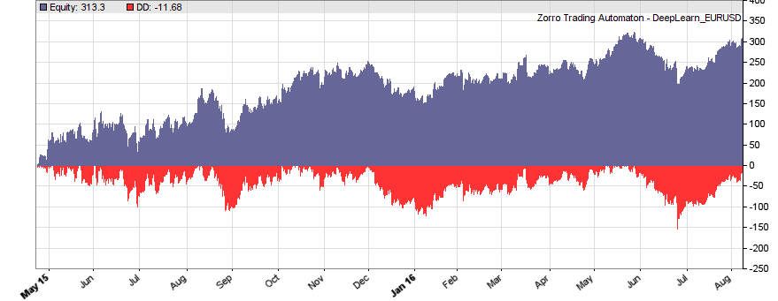
Thank you for this interesting post. I ran it on my pc and obtained similar results as yours. Then I wanted to see if it could perform as well when commission and rollover and slippage were included during test. I used the same figures as the ones used in the workshops and included in the AssetFix.csv file. The modifications I did in your DeepLearn.c file are as follows:
if(Train) {
Hedge = 2;
Spread = RollLong = RollShort = Commission = Slippage = 0;
} else {
Spread = 0.00005;
RollLong = -0.02;
RollShort = 0.01;
Commission = 0.6;
Slippage = 5;
}
The results then were not as optimistic as without commission:
Walk-Forward Test DeepLearn_realistic EUR/USD
Simulated account AssetsFix
Bar period 1 hour (avg 86 min)
Simulation period 09.05.2014-27.01.2017 (16460 bars)
Test period 22.04.2015-27.01.2017 (10736 bars)
Lookback period 100 bars (4 days)
WFO test cycles 18 x 596 bars (5 weeks)
Training cycles 19 x 5367 bars (46 weeks)
Monte Carlo cycles 200
Simulation mode Realistic (slippage 5.0 sec)
Spread 0.5 pips (roll -0.02/0.01)
Commission 0.60
Contracts per lot 1000.0
Gross win/loss 5608$ / -6161$ (-6347p)
Average profit -312$/year, -26$/month, -1.20$/day
Max drawdown -635$ -115% (MAE -636$ -115%)
Total down time 99% (TAE 99%)
Max down time 85 weeks from Jun 2015
Max open margin 40$
Max open risk 41$
Trade volume 10202591$ (5760396$/year)
Transaction costs -462$ spr, 46$ slp, -0.16$ rol, -636$ com
Capital required 867$
Number of trades 10606 (5989/year, 116/week, 24/day)
Percent winning 54.9%
Max win/loss 18$ / -26$
Avg trade profit -0.05$ -0.6p (+11.1p / -14.8p)
Avg trade slippage 0.00$ 0.0p (+1.5p / -1.7p)
Avg trade bars 1 (+1 / -2)
Max trade bars 3 (3 hours)
Time in market 188%
Max open trades 3
Max loss streak 19 (uncorrelated 12)
Annual return -36%
Profit factor 0.91 (PRR 0.89)
Sharpe ratio -1.39
Kelly criterion -5.39
R2 coefficient 0.737
Ulcer index 100.0%
Confidence level AR DDMax Capital
10% -149% 130$ 209$
20% -129% 155$ 241$
30% -119% 170$ 262$
40% -112% 184$ 279$
50% -104% 201$ 301$
60% -95% 220$ 327$
70% -89% 240$ 352$
80% -78% 279$ 403$
90% -70% 310$ 444$
95% -61% 361$ 509$
100% -39% 579$ 793$
Portfolio analysis OptF ProF Win/Loss Wgt% Cycles
EUR/USD .000 0.91 5820/4786 100.0 XX/\XX\X\X/X/\\X\\
EUR/USD:L .000 0.93 2795/2468 39.2 ///\/\\/\//\/\\\\\
EUR/USD:S .000 0.89 3025/2318 60.8 \\/\\/\\\\///\\/\\
I am a very beginner with Zorro, maybe I did a mistake ? What do you think ?
No, your results look absolutely ok. The predictive power of 4 candles is very weak. This is just an experiment for finding out if price action has any predictive power at all.
Although it apparently has, I have not yet seen a really profitable system with this method. From the machine learning systems that we’ve programmed so far, all that turned out profitable used data from a longer price history.
Thank you for the great article, it’s exactly what I needed in order to start experimenting with ML in Zorro.
I’ve noticed that the results are slightly different each time despite using the random seed. Here it doesn’t matter thanks to the large number of trades but for example with daily bars the performance metrics fluctuate much more. My question is: do you happen to know from where does the randomness come? Is it still the training process in R despite the seed?
It is indeed so. Deepnet apparently uses also an internal function, not only the R random function, for randomizing some initial value.
any idea about how to use machine learning like in this example with indicators? you could do as better strategy 6
would be very interesting
Is it grid search inside the neural.train function allowed? I get error when I try it.
Besides Andy, how did you end up definining the LSTM structure using rnn? Is it not clear for me after reading inside the package.
where is the full code?(or where is the repository?)
You said” Use genetic optimization for determining the most important signals just by the most profitable results from the prediction process. Great for curve fitting” How about after using genetic optimization process for determining the most profitable signals , match and measure the most profitable signals with distance metrics/similarity analysis(mutual information,DTW,frechet distance algorithm etc…) then use the distance metrics/similarity analysis as function for neural network prediction? Does that make sense ?
Distance to what? To each other?
Yes find similar profitable signal-patterns in history and find distance between patterns/profitable signals then predict the behavior of the profitable signal in the future from past patterns.
Was wondering about this point you made in Step 5:
“Our target is the return of a trade with 3 bars life time.”
But in the code, doesn’t
Y 0,1,0)
mean that we are actually predicting the SIGN of the return, rather than the return itself?
Yes. Only the binary win/loss result, but not the magnitude of the win or loss is used for the prediction.
“When you used almost 1 year’s data for training a system, it can obviously not deteriorate after a single day. Or if it did, and only produced positive test results with daily retraining, I would strongly suspect that the results are artifacts by some coding mistake.”
There is an additional trap to be aware of related to jcl’s comment above that applies to supervised machine learning techniques (where you train a model against actual outcomes). Assume you are trying to predict the return three bars ahead (as in the example above – LifeTime = 3;). In real time you obviously don’t have access to the outcomes for one, two and three bars ahead with which to retrain your model, but when using historical data you do. With frequently retrained models (especially if using relatively short blocks of training data) it is easy to train a model offline (and get impressive results) with data you will not have available for training in real time. Then reality kicks in. Therefore truncating your offline training set by N bars (where N is the number of bars ahead you are trying to predict) may well be advisable…
Hi Jcl,
Amazing work, could you please share the WFO code as well. I was able to run the code till neural.save but unable to generate the WFO results.
Thank you so much
The code above does use WFO.
Dear jcl, in the text you mentioned that you could predict the current leg of zig-zag indicator, could you please elaborate on how to do that? what features and responses would you reccomend?
I would never claim that I could predict the current leg of zigzag indicator. But we have indeed coded a few systems that attempted that. For this, simply use not the current price movement, but the current zigzag slope as a training target. Which parameters you use for the features is completely up to you.
Hi jcl,
Nice work. I was wondering if you ever tried using something like a net long-short ratio of the asset (I.e. the FXCM SSI index – real time live data) as a feature to improve prediction?
Not with the FXCM SSI index, since it is not available as historical data as far as I know. But similar data of other markets, such as order book content, COT report or the like, have been used as features to a machine learning system.
I see, thanks, and whats’s the experience on those? do they have any predictive power? if you know any materials on this, I would be very interested to read it. (fyi, the SSI index can be exported from FXCM Trading Station (daily data from 2003 for most currency pairs)
Thanks for the info with the SSI. Yes, additional market data can have predictive power, especially from the order book. But since we gathered this experience with contract work for clients, I’m not at liberty to disclose details. However we plan an own study with ML evaluation of additional data, and that might result in an article on this blog.
Thanks jcl, looking forward to it! there is a way to record SSI ratios in a CSV file from a LUA Strategy script (FXCM’s scripting language) for live evaluation. happy to give you some details if you decide to evaluate this. (drop me an email) MyFxbook also has a similar indicator, but no historical data on that one unfortunately.
Hi Jcl,
Does random forest algorithm have any advantage over deep net or neural networks for classification problems in financial data?I make it more clear ; I use number of moving averages and oscillators slope colour change for trading decision(buy -sell-hold).Sometimes one oscillator colour change is lagging other is faster etc..There is no problem at picking tops and bottoms but It is quite challenging to know when to hold.Since random forest doesnt’ need normalization ,do they have any advantage over deep net or neural networks for classification?Thanks.
This depends on the system and the features, so there is no general answer. In the systems we did so far, a random forest or single decision tree was sometimes indeed better than a standard neural network, but a deep network beats anything, especially since you need not care as much about feature preselection. We meanwhile do most ML systems with deep networks.
I see thank you.I have seen some new implementations of LSTM which sounds interesting.One is called phased LSTM another one is from Yarin Gaal.He is using Bayesian technique(gaussian process) as dropout http://www.cs.ox.ac.uk/people/yarin.gal/website/blog_2248.html
Guys,
I hooked up the news flow from forexfactory into this algo and predictive power has improved by 7%.
I downloaded forexfactory news history from 2010. Used a algo to convert that into a value of -1 to 1 for EUR. This value becomes another parameter into the neural training network. I think there is real value there …let me see if we can get the win ratio to 75% and then I thik we have a real winner on hands here. …..
The neural training somehow only yields results with EURUSD.
Anyone tried GBPUSD or EURJPY
That’s also my experience. There are only a few asset types with which price pattern systems seem to really work, and that’s mainly EUR/USD and some cryptos. We also had pattern systems with GBP/USD und USD/JPY, but they work less well and need more complex algos. Most currencies don’t expose patterns at all.
JCL, you are saying “The R script is now controlled by the Zorro script (for this it must have the same name, NeuralLearn.r, only with different extension).”
…same name as what ? Shouldn’t it say DeepLearn.r (instead of NeuralLearn.r) ? Where is the name “NeuralLearn” coming from, we don’t seem to have used it anywhere else. Sorry I am not sure what I am missing here, could you please clarify?
That’s right, DeepLearn.r it is. That was a wrong name in the text. The files in the repository should be correctly named.
Thanks for your reply jcl, much appreciated.
I love your work. And I have got lots to learn.
Hope you don’t mind me asking another question …
Further down you are saying “The neural.save function stores the Models list – it now contains 2 models for long and for short trades – after every training run in Zorro’s Data folder”.
Again, I am not sure why, but I don’t seem to be able to locate that Models list file in the Data folder. In fact it does not seem to make any difference if the neural.save function is there or not. When I [Train] DeepLearn, only the files DeepLearn_EURUSD_x.ml and signals0.csv are being created regardless of whether the function exist or not.
The *.ml files contain the models list.
Hi
Do you have any experience with generative adversarial networks (GANs)?Are they suitable for financial time series ?
We have not yet done a GAN based system. AFAIK GANs are best suited for a different class of problems, not for trading, except maybe in special cases where no immediate success function is available.
I’m getting an error when calling TestOOS() – it seems to hit a problem when trying to generate the confusionMatrix:
Error: `data` and `reference` should be factors with the same levels.
Is this, as JCL mentioned, due to an update in the caret package, and if so, does anyone know how to address this, or perhaps advise of a suitable previous version I could install instead?
Problem solved: it seems there has been a change in caret 6.0-79 that will throw this error.
I installed an earlier version (I went with 6.0-70, however, I think any of them up to and including 6.0-78 should be fine).
Thanks for the info. Possibly the confusionmatrix input format has changed with the last caret version – I’ll check that.
Update: ok, it’s the usual R issue. You must now call it this way:
confusionMatrix(as.factor(Y.pr),as.factor(Y.ob))
@Algo
Can you kindly share your model as i have been struggling to integrate forexfactory data since long.
Hello,
Can you please explain a bit more upon the following function you’re applying…
var change(int n)
{
return scale((priceClose(0) – priceClose(n))/priceClose(0),100)/100;
}
According to the zorro-manual, the function scale takes 2 parameters: scale(var Value, int TimePeriod).
In your function as stated above, you’ve set the value for the variable TimePeriod to 100. What does this mean? What is the influence here?
Does scale implicitely perfoms the following?
for(int i =0; i<100; i++)
{
double array[100];
array[i] = (priceClose(0) – priceClose(i))/priceClose(0);
}
I'm asking because the function 'scale' somewhere needs to retrieve the median value, the P25 and the P75 value from?!
Thanks for explaining a bit more…
Kind regards,
Hans
Almost. scale builds the array in a slightly different way
for(int i =0; i<100; i++)
{
array[i] = (priceClose(i) – priceClose(i+n))/priceClose(i);
...
and then determines the median, P75, P25 of this array for scaling the output.
Hi jcl,
Thanks a lot for this clarification!! Your explanation makes sense indeed… Maybe one additional question… Is there any reason why you opt for scaling / normalizing the input values according to a standard normal (Gaussian) distribution?
Kind regards,
Hans
Only because it’s a standard method. Other normalization methods would probably also work.
Hi,
Thanks for sharing the information, When I expand by adding more candles
confusionMatrix is throwing this error:
Error in !all.equal(nrow(data), ncol(data)) : invalid argument type
If I use same number of candles as in post it works, I’ve been fighting this error for 6 hours now
any help appreciated.
Thanks
KEA
It also seems relevant to number of layers in ‘c’
so this c(50,100,50) works
but this c(100,100,100) throw the error.
Thanks,
//KEA
Call it this way:
confusionMatrix(as.factor(Y.pr),as.factor(Y.ob))
Thanks jcl for the reply,
I actually noticed your comment before and was already using that.
This seems to be very peculiar to the amount of data being sent, I think it’s R issue.
I’m very good at C but still navigating my way with R using zorro help file as a starter.
any pointer appreciated even if not I think you did an amazing job already sharing all of this information
Thanks.
If it also helps, If i examine Y.pr I don’t see the binaries and instead I see this in thousands
………………………
3792 NA
3793 NA
………………..
so probably something wrong has gone with the prediction function.
Yes, I remember that Deepnet had problems with too many layers or neurons. There is a fix somewhere online, but we’re meanwhile using Keras for large nets. The latest Zorro version has this system included with interfaces to other deep learning packages, like Keras/Tensorflow, Mxnet, and H2O. Try Keras.
This is great jcl,
I’m going to download the latest version and give that a go.
I was reading about Keras last night and very glad to see that included.
Thanks so much.
Hello,
thanks for the very interesting article!
i have a question concerning the WFO settings in this experiment.
So for the strategy you set the StartDate=20140601.
And the WFOPeriod=252*60 and Datasplit=90
So the equity curve results start after the 1 year training phase in May 2015.
So out of sample test goes from May 2015 – late 2016
But what i dont understand is why there is during the training phase from 06.2014
also the split between training (90%) and testing (10%) when the out of sample testing comes from May 2015 – late 2016.
For what are these 10 % testing for?
Greetings from Mannheim, Germany
They are for testing the preceding training cycle. Walk forward analysis is explained here: http://manual.zorro-project.com/numwfocycles.htm
yes i read that but what i dont understand is in the machine learning context.
In the strategy all the parameters of the neural net are fixed so i dont get why we test on the 10 % when nothing is optimizing on it.
As i understand it the whole equity curve going from May.15 to 08.16 is a complete out of sample test.
And the time before which is one year (so 252 days with weekends the training of the neural network occurs) is this correct?
This is a walk forward analysis. There are no fixed parameters. A walk forward analysis consists of many test and training cycles. You can look up the concept on Wikipedia and a diagram under the link above.
Can’t say I understand a lot of the comments – very technical stuff.
Very basic ….. the file generated above is
DeepSignals_EURUSD.csv
& NOT
DeepSignalsEURUSD_L.csv
as stated.
The Zorro window states
Train EURUSD_L_DeepSignals_EURUSD.csv
again very basic but where is the file name specified. I tried looking for it when I couldn’t find the file
Yes, this article was from 2016 and file names can have changed in newer Zorro versions. The files are normally in the Data folder.
Thanks a lot for your articles – I find them very inspiring! In the previous post you mentioned that you would describe a trading strategy based on SVMs. Is there a particular reason that you chose deep learning instead? In your experience, does deep learning better generalize than SVMs for trading?
It does indeed. Since I wrote this article, machine learning tools got a lot more powerful and flexible. The new deep learning libraries such as Keras/Tensorflow outperform SVMs in almost all regards.
I see, thank you. Previously, I have experimented with GRUs (RNNs) and TCNs, but haven’t been that happy with it. What do you consider as a good architecture to start with?