
It’s time for the 5th and final part of the Build Better Strategies series. In part 3 we’ve discussed the development process of a model-based system, and consequently we’ll conclude the series with developing a data-mining system. The principles of data mining and machine learning have been the topic of part 4. For our short-term trading example we’ll use a deep learning algorithm, a stacked autoencoder, but it will work in the same way with many other machine learning algorithms. With today’s software tools, only about 20 lines of code are needed for a machine learning strategy. I’ll try to explain all steps in detail.
Our example will be a research project – a machine learning experiment for answering two questions. Does a more complex algorithm – such as, more neurons and deeper learning – produce a better prediction? And are short-term price moves predictable by short-term price history? The last question came up due to my scepticism about price action trading in the previous part of this series. I got several emails asking about the “trading system generators” or similar price action tools that are praised on some websites. There is no hard evidence that such tools ever produced any profit (except for their vendors) – but does this mean that they all are garbage? We’ll see.
Our experiment is simple: We collect information from the last candles of a price curve, feed it in a deep learning neural net, and use it to predict the next candles. My hypothesis is that a few candles don’t contain any useful predictive information. Of course, a nonpredictive outcome of the experiment won’t mean that I’m right, since I could have used wrong parameters or prepared the data badly. But a predictive outcome would be a hint that I’m wrong and price action trading can indeed be profitable.
Machine learning strategy development
Step 1: The target variable
To recap the previous part: a supervised learning algorithm is trained with a set of features in order to predict a target variable. So the first thing to determine is what this target variable shall be. A popular target, used in most papers, is the sign of the price return at the next bar. Better suited for prediction, since less susceptible to randomness, is the price difference to a more distant prediction horizon, like 3 bars from now, or same day next week. Like almost anything in trading systems, the prediction horizon is a compromise between the effects of randomness (less bars are worse) and predictability (less bars are better).
Sometimes you’re not interested in directly predicting price, but in predicting some other parameter – such as the current leg of a Zigzag indicator – that could otherwise only be determined in hindsight. Or you want to know if a certain market inefficiency will be present in the next time, especially when you’re using machine learning not directly for trading, but for filtering trades in a model-based system. Or you want to predict something entirely different, for instance the probability of a market crash tomorrow. All this is often easier to predict than the popular tomorrow’s return.
In our price action experiment we’ll use the return of a short-term price action trade as target variable. Once the target is determined, next step is selecting the features.
Step 2: The features
A price curve is the worst case for any machine learning algorithm. Not only does it carry little signal and mostly noise, it is also nonstationary and the signal/noise ratio changes all the time. The exact ratio of signal and noise depends on what is meant with “signal”, but it is normally too low for any known machine learning algorithm to produce anything useful. So we must derive features from the price curve that contain more signal and less noise. Signal, in that context, is any information that can be used to predict the target, whatever it is. All the rest is noise.
Thus, selecting the features is critical for success – even more critical than deciding which machine learning algorithm you’re going to use. There are two approaches for selecting features. The first and most common is extracting as much information from the price curve as possible. Since you do not know where the information is hidden, you just generate a wild collection of indicators with a wide range of parameters, and hope that at least a few of them will contain the information that the algorithm needs. This is the approach that you normally find in the literature. The problem of this method: Any machine learning algorithm is easily confused by nonpredictive predictors. So it won’t do to just throw 150 indicators at it. You need some preselection algorithm that determines which of them carry useful information and which can be omitted. Without reducing the features this way to maybe eight or ten, even the deepest learning algorithm won’t produce anything useful.
The other approach, normally for experiments and research, is using only limited information from the price curve. This is the case here: Since we want to examine price action trading, we only use the last few prices as inputs, and must discard all the rest of the curve. This has the advantage that we don’t need any preselection algorithm since the number of features is limited anyway. Here are the two simple predictor functions that we use in our experiment (in C):
var change(int n)
{
	return scale((priceClose(0) - priceClose(n))/priceClose(0),100)/100;
}

var range(int n)
{
	return scale((HH(n) - LL(n))/priceClose(0),100)/100;
}
The two functions are supposed to carry the necessary information for price action: per-bar movement and volatility. The change function is the difference of the current price to the price of n bars before, divided by the current price. The range function is the total high-low distance of the last n candles, also in divided by the current price. And the scale function centers and compresses the values to the +/-100 range, so we divide them by 100 for getting them normalized to +/-1. We remember that normalizing is needed for machine learning algorithms.
Step 3: Preselecting predictors
When you have selected a large number of indicators or other signals as features for your algorithm, you must determine which of them is useful and which not. There are many methods for reducing the number of features, for instance:
- Determine the correlations between the signals. Remove those with a strong correlation to other signals, since they do not contribute to the information.
- Compare the information content of signals directly, with algorithms like information entropy or decision trees.
- Determine the information content indirectly by comparing the signals with randomized signals; there are some software libraries for this, such as the R Boruta package.
- Use an algorithm like Principal Components Analysis (PCA) for generating a new signal set with reduced dimensionality.
- Use genetic optimization for determining the most important signals just by the most profitable results from the prediction process. Great for curve fitting if you want to publish impressive results in a research paper.
Reducing the number of features is important for most machine learning algorithms, including shallow neural nets. For deep learning it’s less important, since deep nets with many neurons are normally able to process huge feature sets and discard redundant features. For our experiment we do not preselect or preprocess the features, but you can find useful information about this in articles (1), (2), and (3) listed at the end of the page.
Step 4: Select the machine learning algorithm
R offers many different ML packages, and any of them offers many different algorithms with many different parameters. Even if you already decided about the method – here, deep learning – you have still the choice among different approaches and different R packages. Most are quite new, and you can find not many empirical information that helps your decision. You have to try them all and gain experience with different methods. For our experiment we’ve choosen the Deepnet package, which is probably the simplest and easiest to use deep learning library. This keeps our code short. We’re using its Stacked Autoencoder (SAE) algorithm for pre-training the network. Deepnet also offers a Restricted Boltzmann Machine (RBM) for pre-training, but I could not get good results from it. There are other and more complex deep learning packages for R, so you can spend a lot of time checking out all of them.
How pre-training works is easily explained, but why it works is a different matter. As to my knowledge, no one has yet come up with a solid mathematical proof that it works at all. Anyway, imagine a large neural net with many hidden layers:
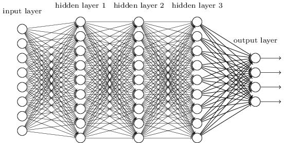
Training the net means setting up the connection weights between the neurons. The usual method is error backpropagation. But it turns out that the more hidden layers you have, the worse it works. The backpropagated error terms get smaller and smaller from layer to layer, causing the first layers of the net to learn almost nothing. Which means that the predicted result becomes more and more dependent of the random initial state of the weights. This severely limited the complexity of layer-based neural nets and therefore the tasks that they can solve. At least until 10 years ago.
In 2006 scientists in Toronto first published the idea to pre-train the weights with an unsupervised learning algorithm, a restricted Boltzmann machine. This turned out a revolutionary concept. It boosted the development of artificial intelligence and allowed all sorts of new applications from Go-playing machines to self-driving cars. Meanwhile, several new improvements and algorithms for deep learning have been found. A stacked autoencoder works this way:
- Select the hidden layer to train; begin with the first hidden layer. Connect its outputs to a temporary output layer that has the same structure as the network’s input layer.
- Feed the network with the training samples, but without the targets. Train it so that the first hidden layer reproduces the input signal – the features – at its outputs as exactly as possible. The rest of the network is ignored. During training, apply a ‘weight penalty term’ so that as few connection weights as possible are used for reproducing the signal.
- Now feed the outputs of the trained hidden layer to the inputs of the next untrained hidden layer, and repeat the training process so that the input signal is now reproduced at the outputs of the next layer.
- Repeat this process until all hidden layers are trained. We have now a ‘sparse network’ with very few layer connections that can reproduce the input signals.
- Now train the network with backpropagation for learning the target variable, using the pre-trained weights of the hidden layers as a starting point.
The hope is that the unsupervised pre-training process produces an internal noise-reduced abstraction of the input signals that can then be used for easier learning the target. And this indeed appears to work. No one really knows why, but several theories – see paper (4) below – try to explain that phenomenon.
Step 5: Generate a test data set
We first need to produce a data set with features and targets so that we can test our prediction process and try out parameters. The features must be based on the same price data as in live trading, and for the target we must simulate a short-term trade. So it makes sense to generate the data not with R, but with our trading platform, which is anyway a lot faster. Here’s a small Zorro script for this, DeepSignals.c:
function run()
{
	StartDate = 20140601; // start two years ago
	BarPeriod = 60; // use 1-hour bars
	LookBack = 100; // needed for scale()

	set(RULES);   // generate signals
	LifeTime = 3; // prediction horizon
	Spread = RollLong = RollShort = Commission = Slippage = 0;

	adviseLong(SIGNALS+BALANCED,0,
		change(1),change(2),change(3),change(4),
		range(1),range(2),range(3),range(4));
	enterLong();
}
We’re generating 2 years of data with features calculated by our above defined change and range functions. Our target is the result of a trade with 3 bars life time. Trading costs are set to zero, so in this case the result is equivalent to the sign of the price difference at 3 bars in the future. The adviseLong function is described in the Zorro manual; it is a mighty function that automatically handles training and predicting and allows to use any R-based machine learning algorithm just as if it were a simple indicator.
In our code, the function uses the next trade return as target, and the price changes and ranges of the last 4 bars as features. The SIGNALS flag tells it not to train the data, but to export it to a .csv file. The BALANCED flag makes sure that we get as many positive as negative returns; this is important for most machine learning algorithms. Run the script in [Train] mode with our usual test asset EUR/USD selected. It generates a spreadsheet file named DeepSignalsEURUSD_L.csv that contains the features in the first 8 columns, and the trade return in the last column.
Step 6: Calibrate the algorithm
Complex machine learning algorithms have many parameters to adjust. Some of them offer great opportunities to curve-fit the algorithm for publications. Still, we must calibrate parameters since the algorithm rarely works well with its default settings. For this, here’s an R script that reads the previously created data set and processes it with the deep learning algorithm (DeepSignal.r):
library('deepnet', quietly = T)
library('caret', quietly = T)

neural.train = function(model,XY)
{
  XY <- as.matrix(XY)
  X <- XY[,-ncol(XY)]
  Y <- XY[,ncol(XY)]
  Y <- ifelse(Y > 0,1,0)
  Models[[model]] <<- sae.dnn.train(X,Y,
      hidden = c(50,100,50),
      activationfun = "tanh",
      learningrate = 0.5,
      momentum = 0.5,
      learningrate_scale = 1.0,
      output = "sigm",
      sae_output = "linear",
      numepochs = 100,
      batchsize = 100,
      hidden_dropout = 0,
      visible_dropout = 0)
}

neural.predict = function(model,X)
{
  if(is.vector(X)) X <- t(X)
  return(nn.predict(Models[[model]],X))
}

neural.init = function()
{
  set.seed(365)
  Models <<- vector("list")
}

TestOOS = function()
{
  neural.init()
  XY <<- read.csv('C:/Zorro/Data/DeepSignalsEURUSD_L.csv',header = F)
  splits <- nrow(XY)*0.8
  XY.tr <<- head(XY,splits);
  XY.ts <<- tail(XY,-splits)
  neural.train(1,XY.tr)
  X <<- XY.ts[,-ncol(XY.ts)]
  Y <<- XY.ts[,ncol(XY.ts)]
  Y.ob <<- ifelse(Y > 0,1,0)
  Y <<- neural.predict(1,X)
  Y.pr <<- ifelse(Y > 0.5,1,0)
  confusionMatrix(Y.pr,Y.ob)
}
We’ve defined three functions neural.train, neural.predict, and neural.init for training, predicting, and initializing the neural net. The function names are not arbitrary, but follow the convention used by Zorro’s advise(NEURAL,..) function. It doesn’t matter now, but will matter later when we use the same R script for training and trading the deep learning strategy. A fourth function, TestOOS, is used for out-of-sample testing our setup.
The function neural.init seeds the R random generator with a fixed value (365 is my personal lucky number). Otherwise we would get a slightly different result any time, since the neural net is initialized with random weights. It also creates a global R list named “Models”. Most R variable types don’t need to be created beforehand, some do (don’t ask me why). The ‘<<-‘ operator is for accessing a global variable from within a function.
The function neural.train takes as input a model number and the data set to be trained. The model number identifies the trained model in the “Models” list. A list is not really needed for this test, but we’ll need it for more complex strategies that train more than one model. The matrix containing the features and target is passed to the function as second parameter. If the XY data is not a proper matrix, which frequently happens in R depending on how you generated it, it is converted to one. Then it is split into the features (X) and the target (Y), and finally the target is converted to 1 for a positive trade outcome and 0 for a negative outcome.
The network parameters are then set up. Some are obvious, others are free to play around with:
- The network structure is given by the hidden vector: c(50,100,50) defines 3 hidden layers, the first with 50, second with 100, and third with 50 neurons. That’s the parameter that we’ll later modify for determining whether deeper is better.
- The activation function converts the sum of neuron input values to the neuron output; most often used are sigmoid that saturates to 0 or 1, or tanh that saturates to -1 or +1.
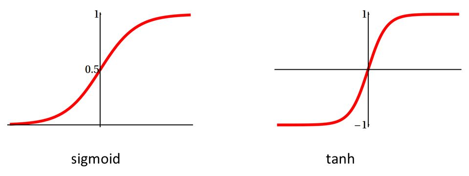
We use tanh here since our signals are also in the +/-1 range. The output of the network is a sigmoid function since we want a prediction in the 0..1 range. But the SAE output must be “linear” so that the Stacked Autoencoder can reproduce the analog input signals on the outputs. Recently in fashion came RLUs, Rectified Linear Units, as activation functions for internal layers. RLUs are faster and partially overcome the above mentioned backpropagation problem, but are not supported by deepnet.
- The learning rate controls the step size for the gradient descent in training; a lower rate means finer steps and possibly more precise prediction, but longer training time.
- Momentum adds a fraction of the previous step to the current one. It prevents the gradient descent from getting stuck at a tiny local minimum or saddle point.
- The learning rate scale is a multiplication factor for changing the learning rate after each iteration (I am not sure for what this is good, but there may be tasks where a lower learning rate on higher epochs improves the training).
- An epoch is a training iteration over the entire data set. Training will stop once the number of epochs is reached. More epochs mean better prediction, but longer training.
- The batch size is a number of random samples – a mini batch – taken out of the data set for a single training run. Splitting the data into mini batches speeds up training since the weight gradient is then calculated from fewer samples. The higher the batch size, the better is the training, but the more time it will take.
- The dropout is a number of randomly selected neurons that are disabled during a mini batch. This way the net learns only with a part of its neurons. This seems a strange idea, but can effectively reduce overfitting.
All these parameters are common for neural networks. Play around with them and check their effect on the result and the training time. Properly calibrating a neural net is not trivial and might be the topic of another article. The parameters are stored in the model together with the matrix of trained connection weights. So they need not to be given again in the prediction function, neural.predict. It takes the model and a vector X of features, runs it through the layers, and returns the network output, the predicted target Y. Compared with training, prediction is pretty fast since it only needs a couple thousand multiplications. If X was a row vector, it is transposed and this way converted to a column vector, otherwise the nn.predict function won’t accept it.
Use RStudio or some similar environment for conveniently working with R. Edit the path to the .csv data in the file above, source it, install the required R packages (deepnet, e1071, and caret), then call the TestOOS function from the command line. If everything works, it should print something like that:
> TestOOS()
begin to train sae ......
training layer 1 autoencoder ...
####loss on step 10000 is : 0.000079
training layer 2 autoencoder ...
####loss on step 10000 is : 0.000085
training layer 3 autoencoder ...
####loss on step 10000 is : 0.000113
sae has been trained.
begin to train deep nn ......
####loss on step 10000 is : 0.123806
deep nn has been trained.
Confusion Matrix and Statistics

          Reference
Prediction    0    1
         0 1231  808
         1  512  934

               Accuracy : 0.6212
                 95% CI : (0.6049, 0.6374)
    No Information Rate : 0.5001
    P-Value [Acc > NIR] : < 2.2e-16

                  Kappa : 0.2424
 Mcnemar's Test P-Value : 4.677e-16

            Sensitivity : 0.7063
            Specificity : 0.5362
         Pos Pred Value : 0.6037
         Neg Pred Value : 0.6459
             Prevalence : 0.5001
         Detection Rate : 0.3532
   Detection Prevalence : 0.5851
      Balanced Accuracy : 0.6212

       'Positive' Class : 0

>
TestOOS reads first our data set from Zorro’s Data folder. It splits the data in 80% for training (XY.tr) and 20% for out-of-sample testing (XY.ts). The training set is trained and the result stored in the Models list at index 1. The test set is further split in features (X) and targets (Y). Y is converted to binary 0 or 1 and stored in Y.ob, our vector of observed targets. We then predict the targets from the test set, convert them again to binary 0 or 1 and store them in Y.pr. For comparing the observation with the prediction, we use the confusionMatrix function from the caret package.
A confusion matrix of a binary classifier is simply a 2×2 matrix that tells how many 0’s and how many 1’s had been predicted wrongly and correctly. A lot of metrics are derived from the matrix and printed in the lines above. The most important at the moment is the 62% prediction accuracy. This may hint that I bashed price action trading a little prematurely. But of course the 62% might have been just luck. We’ll see that later when we run a WFO test.
A final advice: R packages are occasionally updated, with the possible consequence that previous R code suddenly might work differently, or not at all. This really happens, so test carefully after any update.
Step 7: The strategy
Now that we’ve tested our algorithm and got some prediction accuracy above 50% with a test data set, we can finally code our machine learning strategy. In fact we’ve already coded most of it, we just must add a few lines to the above Zorro script that exported the data set. This is the final script for training, testing, and (theoretically) trading the system (DeepLearn.c):
#include <r.h>

function run()
{
	StartDate = 20140601;
	BarPeriod = 60;	// 1 hour
	LookBack = 100;

	WFOPeriod = 252*24; // 1 year
	DataSplit = 90;
	NumCores = -1;  // use all CPU cores but one

	set(RULES);
	Spread = RollLong = RollShort = Commission = Slippage = 0;
	LifeTime = 3;
	if(Train) Hedge = 2;

	if(adviseLong(NEURAL+BALANCED,0,
		change(1),change(2),change(3),change(4),
		range(1),range(2),range(3),range(4)) > 0.5)
		enterLong();
	if(adviseShort() > 0.5)
		enterShort();
}
We’re using a WFO cycle of one year, split in a 90% training and a 10% out-of-sample test period. You might ask why I have earlier used two year’s data and a different split, 80/20, for calibrating the network in step 5. This is for using differently composed data for calibrating and for walk forward testing. If we used exactly the same data, the calibration might overfit it and compromise the test.
The selected WFO parameters mean that the system is trained with about 225 days data, followed by a 25 days test or trade period. Thus, in live trading the system would retrain every 25 days, using the prices from the previous 225 days. In the literature you’ll sometimes find the recommendation to retrain a machine learning system after any trade, or at least any day. But this does not make much sense to me. When you used almost 1 year’s data for training a system, it can obviously not deteriorate after a single day. Or if it did, and only produced positive test results with daily retraining, I would strongly suspect that the results are artifacts by some coding mistake.
Training a deep network takes really a long time, in our case about 10 minutes for a network with 3 hidden layers and 200 neurons. In live trading this would be done by a second Zorro process that is automatically started by the trading Zorro. In the backtest, the system trains at any WFO cycle. Therefore using multiple cores is recommended for training many cycles in parallel. The NumCores variable at -1 activates all CPU cores but one. Multiple cores are only available in Zorro S, so a complete walk forward test with all WFO cycles can take several hours with the free version.
In the script we now train both long and short trades. For this we have to allow hedging in Training mode, since long and short positions are open at the same time. Entering a position is now dependent on the return value from the advise function, which in turn calls either the neural.train or the neural.predict function from the R script. So we’re here entering positions when the neural net predicts a result above 0.5.
The R script is now controlled by the Zorro script (for this it must have the same name, DeepLearn.r, only with different extension). It is identical to our R script above since we’re using the same network parameters. Only one additional function is needed for supporting a WFO test:
neural.save = function(name)
{
  save(Models,file=name)
}
The neural.save function stores the Models list – it now contains 2 models for long and for short trades – after every training run in Zorro’s Data folder. Since the models are stored for later use, we do not need to train them again for repeated test runs.
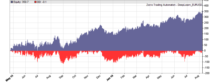
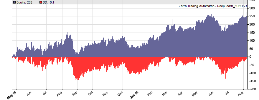
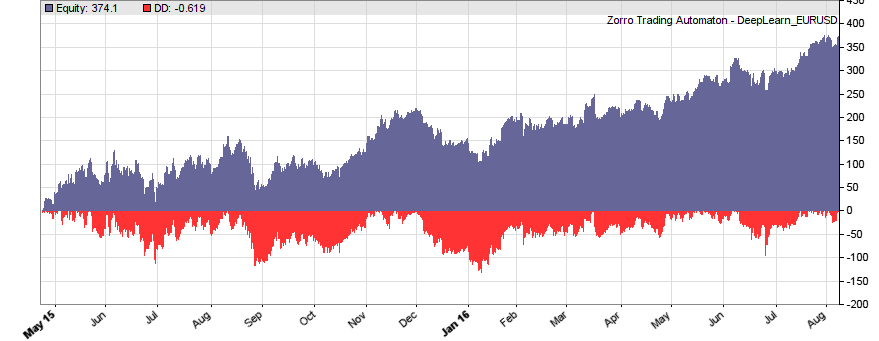
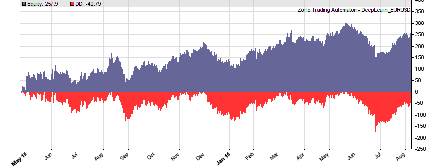
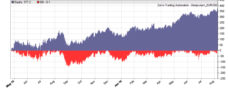
This is the WFO equity curve generated with the script above (EUR/USD, without trading costs):
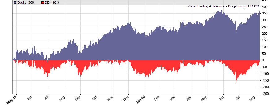
Although not all WFO cycles get a positive result, it seems that there is some predictive effect. The curve is equivalent to an annual return of 89%, achieved with a 50-100-50 hidden layer structure. We’ll check in the next step how different network structures affect the result.
Since the neural.init, neural.train, neural.predict, and neural.save functions are automatically called by Zorro’s adviseLong/adviseShort functions, there are no R functions directly called in the Zorro script. Thus the script can remain unchanged when using a different machine learning method. Only the DeepLearn.r script must be modified and the neural net, for instance, replaced by a support vector machine. For trading such a machine learning system live on a VPS, make sure that R is also installed on the VPS, the needed R packages are installed, and the path to the R terminal set up in Zorro’s ini file. Otherwise you’ll get an error message when starting the strategy.
Step 8: The experiment
If our goal had been developing a strategy, the next steps would be the reality check, risk and money management, and preparing for live trading just as described under model-based strategy development. But for our experiment we’ll now run a series of tests, with the number of neurons per layer increased from 10 to 100 in 3 steps, and 1, 2, or 3 hidden layers (deepnet does not support more than 3). So we’re looking into the following 9 network structures: c(10), c(10,10), c(10,10,10), c(30), c(30,30), c(30,30,30), c(100), c(100,100), c(100,100,100). For this experiment you need an afternoon even with a fast PC and in multiple core mode. Here are the results (SR = Sharpe ratio, R2 = slope linearity):
| * 10 neurons | * 30 neurons | * 100 neurons | |
| 1 |
 |
 |
 |
| 2 |
 |
 |
 |
| 3 |
 |
 |
 |
We see that a simple net with only 10 neurons in a single hidden layer won’t work well for short-term prediction. Network complexity clearly improves the performance, however only up to a certain point. A good result for our system is already achieved with 3 layers x 30 neurons. Even more neurons won’t help much and sometimes even produce a worse result. This is no real surprise, since for processing only 8 inputs, 300 neurons can likely not do a better job than 100.
Conclusion
Our goal was determining if a few candles can have predictive power and how the results are affected by the complexity of the algorithm. The results seem to suggest that short-term price movements can indeed be predicted sometimes by analyzing the changes and ranges of the last 4 candles. The prediction is not very accurate – it’s in the 58%..60% range, and most systems of the test series become unprofitable when trading costs are included. Still, I have to reconsider my opinion about price action trading. The fact that the prediction improves with network complexity is an especially convincing argument for short-term price predictability.
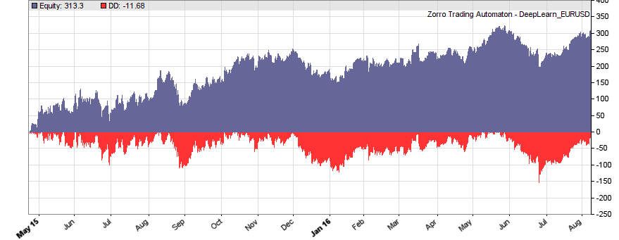
It would be interesting to look into the long-term stability of predictive price patterns. For this we had to run another series of experiments and modify the training period (WFOPeriod in the script above) and the 90% IS/OOS split. This takes longer time since we must use more historical data. I have done a few tests and found so far that a year seems to be indeed a good training period. The system deteriorates with periods longer than a few years. Predictive price patterns, at least of EUR/USD, have a limited lifetime.
Where can we go from here? There’s a plethora of possibilities, for instance:
- Use inputs from more candles and process them with far bigger networks with thousands of neurons.
- Use oversampling for expanding the training data. Prediction always improves with more training samples.
- Compress time series f.i. with spectal analysis and analyze not the candles, but their frequency representation with machine learning methods.
- Use inputs from many candles – such as, 100 – and pre-process adjacent candles with one-dimensional convolutional network layers.
- Use recurrent networks. Especially LSTM could be very interesting for analyzing time series – and as to my knowledge, they have been rarely used for financial prediction so far.
- Use an ensemble of neural networks for prediction, such as Aronson’s “oracles” and “comitees”.
Papers / Articles
(1) A.S.Sisodiya, Reducing Dimensionality of Data
(2) K.Longmore, Machine Learning for Financial Prediction
(3) V.Perervenko, Selection of Variables for Machine Learning
(4) D.Erhan et al, Why Does Pre-training Help Deep Learning?
I’ve added the C and R scripts to the 2016 script repository. You need both in Zorro’s Strategy folder. Zorro version 1.474, and R version 3.2.5 (64 bit) was used for the experiment, but it should also work with other versions.
It depends on the signals that you are processing. We experimented with LSTMs and with 1D convolutional stages.
(Belated) Thanks for a highly informative article! You know, I am wondering if TestOOS is skewing the results: By setting the SIGNALS+BALANCED flag, the test data XY.ts is also becoming balanced, which in reality of course it wouldn’t be.
When I removed duplicates in XY.ts, in my experiments the accuracy dropped from 62% to about 52%.
Or am I on the wrong track here?
No, you’re right. The test data is balanced and removing duplicates out of it can of course increase or reduce the accuracy, even strongly with small data sets. For a confusion matrix, balanced test data is normally preferable. For other purposes it may be unpreferable or not matter.
Thanks for this series of articles.
But in relation to his comment “I got several emails asking about the“ trading system generators ”or similar price action tools that are praised on some websites. There is no hard evidence that such tools ever produced any profit (except for their vendors) – but does this mean that they are all garbage? We’ll see. ”
What opinion do you have regarding the software: Trading System Lab and Genetic System Builder.
Systems created in both softwares reached the top ten of Futures Truth magazine in 2018
I don’t know Trading System Lab and Genetic System Builder, but there are hundreds of similar tools around. So I can’t honestly say if they have any value or if the appearance in that magazine has any meaning.
Thanks, Jcl, for a great post and a great blog! Unfortunately, it is obvious that the average profit per trade of this particular strategy is too low to make any money in real life. Also, it is interesting to notice that the accuracy of the DeepNet predictions is higher than the number of winning trades in Zorro. I posted something about that here: https://zorro-trader.co/zorro-trader-how-accurate-is-deepnet/
I guess sometimes the marker gremlins are eating our lunch…
How much accuracy is enough to cover spread and trading costs?
Depends on asset and broker, but it should be well above 55.
This series of articles “Build Better Strategies” that was made in 2016 needs to be updated?
perhaps there are a new series more updated or as a base is still valid.
Thanks
Referencing program ‘Alice4a’ in chapter 6 of your book, if I want to use a pattern with 5 candles, where the total number of signals is higher than 20 for the adviseLong(), and I would need to store the signals in an array, does the ordering of the signals within the array matter? Should the signals place in an order such that they will be divided into pattern groups that I desired? Thanks.
The signal limit for patterns is 20. Patterns with 5 candles are theoretically possible, since they have only 15 signals. But I don’t think that you will find any useful patterns of more than 3 candles.
Thanks for your reply. Based on Zorro Help page for the adviseLong(): “adviseLong (int Method, var Objective, var* Signals, int NumSignals): var”, the var array ‘Signals’ can has more than 20 signals.
Does the ‘ordering’ of the signals within the array ‘Signals’ matter? as far as creating difference pattern groups for the machine learning? Thanks.
The order does matter when you group the signals, as in the example. The limit is really 20, even when the array has more signals. You can believe me, I have programmed this function ;).