
This indicator can improve – sometimes even double – the profit expectancy of trend following systems. The Market Meanness Index tells whether the market is currently moving in or out of a “trending” regime. It can this way prevent losses by false signals of trend indicators. It is a purely statistical algorithm and not based on volatility, trends, or cycles of the price curve.
There are already several methods for differentiating trending and nontrending market regimes. Some of them are rumored to really work, at least occasionally. John Ehlers proposed the Hilbert Transform or a Cycle / Trend decomposition, Benoit Mandelbrot the Hurst Exponent. In comparison, the source code of the Market Meanness Index is relatively simple:
// Market Meanness Index
double MMI(double *Data,int Length)
{
  double m = Median(Data,Length);
  int i, nh=0, nl=0;
  for(i=1; i<Length; i++) {
    if(Data[i] > m && Data[i] > Data[i-1]) // mind Data order: Data[0] is newest!
      nl++;
    else if(Data[i] < m && Data[i] < Data[i-1])
      nh++;
  }
  return 100.*(nl+nh)/(Length-1);
}
This code is in C for Zorro, but meanwhile also versions for MT4, Amibroker, Ninja Trader, and other platforms have been programmed by users. As the name suggests, the indicator measures the meanness of the market – its tendency to revert to the mean after pretending to start a trend. If that happens too often, all trend following systems will bite the dust.
The Three-Quarter Rule
Any series of independent random numbers reverts to the mean – or more precisely, to their median – with a probability of 75%. Assume you have a sequence of random, uncorrelated daily data – for instance, the daily rates of change of a random walk price curve. If Monday’s data value was above the median, then in 75% of all cases Tuesday’s data will be lower than Monday’s. And if Monday was below the median, 75% chance is that Tuesday will be higher. The proof of the 75% rule is relatively simple and won’t require integral calculus. Consider a data series with median M. By definition, half the values are less than M and half are greater (for simplicity’s sake we’re ignoring the case when a value is exactly M). Now combine the values to pairs each consisting of a value Py and the following value Pt. Thus each pair represents a change from Py to Pt. We now got a lot of changes that we divide into four sets:
- (Pt < M, Py < M)
- (Pt < M, Py > M)
- (Pt > M, Py < M)
- (Pt > M, Py > M)
These four sets have obviously the same number of elements – that is, 1/4 of all Py->Pt changes – when Pt and Py are uncorrelated, i.e. completely independent of one another. The value of M and the kind of data in the series won’t matter for this. Now how many data pairs revert to the median? All pairs that fulfill this condition: (Py < M and Pt > Py) or (Py > M and Pt < Py) The condition in the first bracket is fulfilled for half the data in set 1 (in the other half is Pt less than Py) and in the whole set 3 (because Pt is always higher than Py in set 3). So the first bracket is true for 1/2 * 1/4 + 1/4 = 3/8 of all data changes. Likewise, the second bracket is true in half the set 4 and in the whole set 2, thus also for 3/8 of all data changes. 3/8 + 3/8 yields 6/8, i.e. 75%. This is the three-quarter rule for random numbers.
The MMI function just counts the number of data pairs for which the conditition is met, and returns their percentage. The Data series may contain prices or price changes. Prices have always some serial correlation: If EUR / USD today is at 1.20, it will also be tomorrow around 1.20. That it will end up tomorrow at 70 cents or 2 dollars per EUR is rather unlikely. This serial correlation is also true for a price series calculated from random numbers, as not the prices themselves are random, but their changes. Thus, the MMI function should return a smaller percentage, such as 55%, when fed with prices.
Unlike prices, price changes have not necessarily serial correlation. A one hundred percent efficient market has no correlation between the price change from yesterday to today and the price change from today to tomorrow. If the MMI function is fed with perfectly random price changes from a perfectly efficient market, it will return a value of about 75%. The less efficient and the more trending the market becomes, the more the MMI decreases. Thus a falling MMI is a indicator of an upcoming trend. A rising MMI hints that the market will get nastier, at least for trend trading systems.
Using the MMI in a trend strategy
One could assume that MMI predicts the price direction. A high MMI value indicates a high chance of mean reversion, so when prices were moving up in the last time and MMI is high, can we expect a soon price drop? Unfortunately it doesn’t work this way. The probability of mean reversion is not evenly distributed over the Length of the Data interval. For the early prices it is high (since the median is computed from future prices), but for the late prices, at the very time when MMI is calculated, it is down to just 50%. Predicting the next price with the MMI would work as well as flipping a coin.
Another mistake would be using the MMI for detecting a cyclic or mean-reverting market regime. True, the MMI will rise in such a situation, but it will also rise when the market becomes more random and more effective. A rising MMI alone is no promise of profit by cycle trading systems.
So the MMI won’t tell us the next price, and it won’t tell us if the market is mean reverting or just plain mean, but it can reveal information about the success chance of trend following. For this we’re making an assumption: Trend itself is trending. The market does not jump in and out of trend mode suddenly, but with some inertia. Thus, when we know that MMI is rising, we assume that the market is becoming more efficient, more random, more cyclic, more reversing or whatever, but in any case bad for trend trading. However when MMI is falling, chances are good that the next beginning trend will last longer than normal.
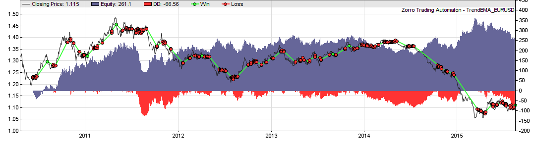
This way the MMI can be an excellent trend filter – in theory. But we all know that there’s often a large gap between theory and practice, especially in algorithmic trading. So I’m now going to test what the Market Meanness Index does to the collection of the 900 trend following systems that I’ve accumulated. For a first quick test, this was the equity curve of one of the systems, TrendEMA, without MMI (44% average annual return):
This is the same system with MMI (55% average annual return):
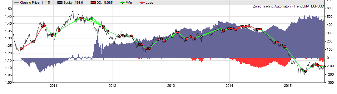
We can see that the profit has doubled, from $250 to $500. The profit factor climbed from 1.2 to 1.8, and the number of trades (green and red lines) is noticeable reduced. On the other hand, the equity curve started with a drawdown that wasn’t there with the original system. So MMI obviously does not improve all trades. And this was just a randomly selected system. If our assumption about trend trendiness is true, the indicator should have a significant effect also on the other 899 systems.
This experiment will be the topic of the next article, in about a week. As usually I’ll include all the source code for anyone to reproduce it. Will the MMI miserably fail? Or improve only a few systems, but worsen others? Or will it light up the way to the Holy Grail of trend strategies? Let the market be the judge.
Next: Testing the Market Meanness Index
Addendum (2022). I thought my above proof of the 3/4 rule was trivial and no math required, but judging from some comments, it is not so. The rule appears a bit counter-intuitive at first glance. Some comments also confuse a random walk (for example, prices) with a random sequence (for example, price differences). Maybe I have just bad explained it – in that case, read up the proof anywhere else. I found the two most elaborate proofs of the 3/4 rule, geometrical and analytical, in this book:
(1) Andrew Pole, Statistical Arbitrage, Wiley 2007
And with no reading and no math: Take a dice, roll it 100 times, write down each result, get the median of all, and then count how often a pair reverted to the median.
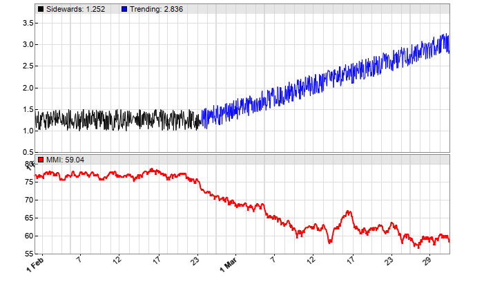
Below you can see the MMI applied to a synthetic price curve, first sidewards (black) and then with added trend (blue). For using the MMI with real prices or price differences, read the next article.
The code:
function run()
{
	BarPeriod = 60;
	MaxBars = 1000;
	LookBack = 500;
	asset(""); // dummy asset
	ColorUp = ColorDn = 0; // don't plot a price curve
	set(PLOTNOW);

	if(Init) seed(1000);
	int TrendStart = LookBack + 0.4*(MaxBars-LookBack);
	vars Signals = series(1 + 0.5*genNoise());
	if(Bar > TrendStart)
		Signals[0] += 0.003*(Bar-TrendStart);
	int Color = RED;
	int TimePeriod = 0.5*LookBack;
	if(Bar < TrendStart)
		plot("Sidewards",Signals,MAIN,BLACK);
	else
		plot("Trending",Signals,MAIN,BLUE);
	plot("MMI",MMI(Signals,TimePeriod),NEW|LINE,Color);
}
There are some links in the page which does not work. As “next page” in some cases.
There are some indicators which try to find trend more. Did you consider to do an analysis of all of them as you did with the trend indicators. I mean instead of just using MMI to the 900 systems, you could use another ones by using the same approach.
I can certainly test other trend indicators, as this requires only a small change of the script. But I don’t know many that promise to really work. Which indicator do you have in mind?
I dont have any really in mind. You mention above Hurst and Hilbert Transform and so on. I like the methodology you use to find out which trend indicator is actually better. I was wondering what would be the result if you use the same methodology to find out if the market is in trend mode by using different indicators and not just MMI.
Yes, I’ll test more filters and also the more conventional crossover rather than peaks and valleys for trend systems. The MMI already produces pretty good results, but it can not harm to test as many algorithms as possible. However the next planned experiment is with a “deep learning” network.
Well congratulations again for this amazing blog. Really inspiring as well.
I wonder if you can keep aplying this kind of approach in the next steps of strategy development like one can lock the best filter found so far and use instead as a variable input different kind of money management functions for example.
Nice article; I’m looking forward to trying this out sometime. Also, I love the name of your blog.
Um, isnt there lookahead bias here? the median is computed over the entire data set. Not sure it can be used at any point in the data set to make a decision, as is.
Ah, you really looked in the code! If the median was computed from future data, it would indeed be lookahead bias. But all data is from the past and available when calling the function. You can anyway not look ahead with the Zorro platform, except when you set a certain flag that allows access to future data. Otherwise it produces a warning message.
Hey! I’m enjoying the blog
There seems to be an unnecessary restriction on your test for mean reversion vs trend. Why must the price be beyond the median before measuring which direction it goes? “Mean reversion” usually is referring to a more general ‘where prices really ought to be’ rather than the mathematical mean (or in your case, median). Wouldn’t a more appropriate trend-vs-mean-reversion system simply look at auto-correlation? If a price moves one direction and then back the other way, regardless of its relative position to the median, then it would be considered “reverting”. This doesn’t invalidate your approach, but insisting that noise is mean-reverting 75% of the time isn’t describing the reality accurately. Really you’re saying “noise moving away from the median tends to move back toward the median 75% of the time.” Or did I misunderstand?
Thanks!
I think you understood it correctly – your formulation is indeed more accurate. The MMI is not really intended for distinguishing between mean reversion and trend. For this f.i. the Hurst Exponent produces better results, at least according to my experiences. The MMI works however well for determining just the presence or absence of trend. As soon as it begins to return high values in the 75% area, it can be the begin of mean reversion or it can be just randomness – the MMI can not distinguish that. Both situations are likewise bad for trend following.
Based on your post I have programmed and tested MMI on Quantopian. I choose different stocks (SPY, BAC, AAPL, NFLX, etc) daily close price changes and different MMI lengths (100,200,300,500) . The testing date range was from 01/01/2012 to 01/14/2016.
The result was always around 75% There was no value under 70% and above 85% in any case.
For example:
SPY
from 01/01/2012 to 01/14/2016
MMI length 300
Average: 76.092%
Standard deviation: 1.716
Max:80.27%
Min:71.91%
Is this a good result?
It seems to me that MMI is not usable or just this small changes under 75% what I should follow?
If I used prices instead of price changes, the result was always around 50%, the standard deviation was higher, but not so convincing.
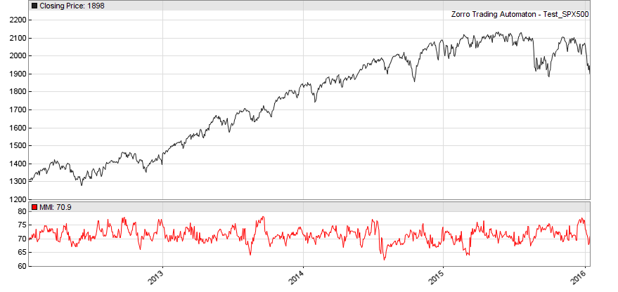
Yes, this is a good result when you tested daily returns, which are normally not significantly trending. Even a bit mean reverting before mid-2014. You should get such a curve:
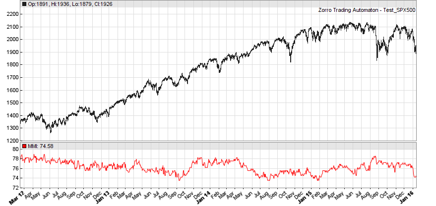
But as soon as you look into hour returns, you’ll see more trendiness:
The script:
void run() { StartDate = 20120101; EndDate = 2016; plot("MMI", MMI(series(priceClose(0)-priceClose(1)),300), NEW, RED); }Thank you for your quick answer.
So all trend following systems based on daily close prices are doomed.
In case of 1H or forex my hypothesis is that these continuous, connected data in time and so more trendiness. Between daily close prices there are a big gap in time after the market closes and next day opens.
So maybe I should trade on shorter time scale or on forex.
“So when you look at a random data sequence, if Monday’s data was above the median, in 75% of all cases Tuesday’s data is lower than Monday’s”
In a random price sequence, the chance of going higher/lower at each point is *always* 50% – irrespective of where the mean lies or what happened yesterday.
This is indeed a frequent misconception. The chance of going higher/lower at a certain point is very different to the chance of a price pair in a random sequence to revert to the median. If you do not believe the proof above, just run the script and look at the results. And if you do not believe the script either, roll the dice a hundred times, write down all the numbers, and count how often subsequent numbers revert to the median. 🙂
“If you do not believe the proof above, just run the script and look at the results”
So the snippet below is a Python transcription of the above run over a random walk sequence.
The MMI is always 50% Why the difference?
import random
import numpy
def random_walk(n):
seq = [0]
for i in range(n):
if random.random() > 0.5:
seq.append( seq[-1] + 1 )
else:
seq.append( seq[-1] – 1 )
return seq
def market_meanness_index(data):
m = numpy.median(data)
nh = nl = 0
for i in range(1, len(data)):
if data[i] > m and data[i] > data[i-1]:
nl += 1
elif data[i] < m and data[i] < data[i-1]:
nh += 1
return 100.0 * (nl+nh) / (len(data)-1)
mmi = market_meanness_index(random_walk(10**6))
print "{:.1f}%".format(mmi)
Because your random walk is not a random sequence. A random walk has serial correlation. A correct random sequence would be:
def random_walk(n):
seq = [0]
for i in range(n):
seq.append(random.random())
return seq
The same goes for price data: prices are not random. They have serial correlation. But price changes are random, at least in a perfect efficient market.
That makes sense! Thanks for the clarification and the prompt responses.
Hi, can you please explain the detail algorithm that how MMI helps in trend detection? Or some pseudo code. Though I found you check “falling” in the other blog, I don’t know how “falling” works.
Thanks
I think the algorithm is explained above under “The three-quarter rule”. If something is unclear, just ask. The MMI detects trend indirectly, by absence of mean reversion. “Falling” is a binary function that just determines if a data series is rising or falling.
@Mathafarn and anyone who wants to have a look at MMI for Python, the python version shown is not the same as Zorros version.
First of all np.median() isn’t the same as the median Zorro uses, second the for-loop is going the wrong way leading to different results.
Here’s a fixed version:
def market_meanness_index(data):
data_sorted = sorted(data)
if len(data) % 2:
m = data_sorted[int(len(data) / 2)]
else:
m = (data_sorted[int(len(data_sorted) / 2)+1] + data_sorted[int(len(data_sorted) / 2)]) / 2.0
nh = nl = 0
for i in range(0, len(data)-1):
if data[i] > m and data[i] > data[i+1]:
nl += 1
elif data[i] < m and data[i] < data[i+1]:
nh += 1
return 100.0 * (nl+nh) / (len(data)-1)
Hi jcl,
Great job!
Several quick questions
1. About the application of MMI, can we use percentile(MMI,25), if today’s MMI is lower than 25%, we say market is in trend, otherwise, not.
2. Which ones are sound indicators for determining market regime?
3. Some markets are easier to generate profit from than others, I call them more “tradable”, just like what you found in this experiment that SPY is the most noisy market while commodities are more trendy, any indicators on this?
Thank you
Jeff
1. Yes, a percentile threshold would certainly make sense.
2. For instance the Hurst Exponent – a fellow blogger, Robot Wealth, has recently written an article about it.
3. Theoretically, an indicator like Shannon Entropy could be used for determining more randomness or more tradeability in a market. This could be an interesting topic for research.
The python example below tests a perfect trend and a perfect mean reversion data sequence. The MMI for both is 50%. Why is this? Thanks….
import math
import numpy
def market_meanness_index(data):
m = numpy.median(data)
nh = nl = 0
for i in range(1, len(data)):
if data[i] > m and data[i] > data[i-1]:
nl += 1
elif data[i] < m and data[i] < data[i-1]:
nh += 1
return 100.0*(nl+nh)/(len(data)-1)
# perfect trend: MMI 50%
trend_data = numpy.arange(0.0, math.pi, 0.01)
print market_meanness_index(trend_data)
# perfect mean reversion: MMI 50%
sin_data = map(lambda x: math.sin(x), trend_data)
print market_meanness_index(sin_data)
Because you sampled not a sine curve, but its slope, which is in fact a perfect trend. A flat trend will always produce about 50%, but a sine curve must be sampled over several periods for being mean reverting. It then produces a MMI in the 60% or 70% area, as you can see below.
function run(){
MaxBars = 1500;
LookBack = 100;
asset(""); // dummy asset
vars Data1 = series(genSine(5));
plot("Sine",Data1,NEW,BLACK);
plot("MMI_Sine",MMI(Data1,100),NEW,BLACK);
vars Data2 = series(Bar*0.01);
plot("Trend",Data2,NEW,BLACK);
plot("MMI_Trend",MMI(Data2,100),NEW,BLACK);
}
Thanks for the excellent article. Would MMI be useful to prevent losses in am mean reverting strategy or which other indocator would you recommend? Thank you.
No, the MMI will probably not work well for filtering mean reverting trades, since it makes no difference between “less trendy” and “more random”. For filtering mean reversion I would try to detect the dominant cycle – mean reversion is normally related to some short-term cyclic behavior – and check the amplitude of the dominant frequency component.
Thanks, will look into that.
Hi jcl! Do you happen to have the MetaTrader version of this? Every time I try to access the link you posted I get an error message.
Also do you happen to know if anyone has coded this for Tradestation?
It’s some time ago, but if I remember right someone posted a MT4 version on Steve Hopwood’s forum. There was also a Tradestation version, but I cannot remember the link anymore. It should be anyway relatively easy to port the code to Tradestation.
I tried to translate the MMI into Easylanguage. But I always just get a steadily increasing line.
nl and nh are always increasing values?
I’m no Easylanguage expert, but AFAIK it has no local variables, anything is global. If so, then make sure that nl and nh are reset to zero at the begin of the function.
If I reset nl and nh at each bar, I get a binary wave between 0 and 0.33.
Do I have to loop the calculation? For how long?
You should get about 0.75 when you test with random numbers. With 0.33, something is wrong. The indicator is not cumulative, so you need not loop it.
if nl and nh get reset every bar and the indicator is not cumulative, the formula would always be
100*1/299
as nl or nh are always 1
Could you maybe paraphrase the formula in pseudo-code, in case I misread the C-code?
I don’t know if it helps, but anyway:
count all price decreases above the median
add all price increases below the median
divide by the number of prices and return the percentage.
Hacker’s first rule: Code only what you understand.
>>jcl says:
>>July 18, 2017 at 10:11
>>It’s some time ago, but if I remember right someone posted a MT4 version on Steve Hopwood’s forum.
>>There was also a Tradestation version, but I cannot remember the link anymore. It should be
>>anyway relatively easy to port the code to Tradestation.
The MT4 version was on this link, but it seems to be deleted:
http://www.stevehopwoodforex.com/phpBB3/viewtopic.php?uid=17&f=27&t=3714&start=0
Maybe someone still has the indicator for MT4 or Tradestation
I have translated the indicator, but it looks quite different from your example
http://imgur.com/a/WWD0O
calculated on close of daily bars, length 300
Seems like it’s high, when trending and low when mean reverting. Also highest value is 60%
Then apparently the translation was still not a real success. You must get the same curve, and trending produces lower, not higher values.
but the calculation base is correct? length 300 on daily close, compared to median?
Yes. But make sure that you get the data order right. It’s a financial series, with the newest data at the begin. If the order is wrong, rising and falling is swapped.
you mean it would be different if the counter of true conditions is increasing (from old to new data) from looking back from the current bar to the last 300 bars?
Look at the code. Changing the data order is equivalent to swapping two of the four ‘>’ and ‘<' operators.
Hi, I have a question about price changes being used in this indicator. I have found a version that uses open[0] – close[0] to represent the price change.
Is that accurate or should we use close[0] – close[1] as the price change?
Does it mater or could I use any highl0] – low[0].
Also I have seen this indicator coded incorrectly rather than using the median which is the middle of a price series some versions are using the average ( arithmetic mean). F
Will that use adversely effect the calculation?
close[0]-close[1] is the correct price change. It won’t make a difference for 24h traded assets, but can produce a different result for stocks. And the average is wrong. It must be really the median.
I’m backtesting MMI in a set of prices where I clearly see a downtrend. I’m getting an MMI of 40 if I test it with prices, and an MMI of 48 if I test it with price change. I guess that it means that the market is in a strong tendency. Am I right?
So, could we say that the lower the MMI, the better for trend trading systems? So if we find three markets with values 30, 20, and 10 , would be the last one the better for a trend trading strategy?
Well, I guess I talked too soon, sorry for that. Now, I’m trying to analyze MMI within a 30m strategy ; with a list of 404 price changes, completely sideways (https://imgur.com/a/ggwJ3), I’m getting a MMI of 50.49; If instead I use the close prices, I’m getting a MMI of 48.76. In this case obviously the price is not in a trend because it goes up & down.
An MMI of 48 means a strong trend in the tested period (or a wrong MMI implementation). On normal trending price curves the MMI is in the area of 60-70.
I’m going to paste the MMI code (python + pandas) also for the records, it may be useful for someone else (I think the code is ok but I may be wrong!). What I don’t get is why I’m getting a similar result (around 45-50) if the curve price is a “mountain” (trend up and then down) or if it is just an uptrend
def MMI(df):
m = df.Close.median()
length = len(df.index)
nh=0
nl=1
df.loc[0,”nl”] = 0
df.loc[0,”nh”] = 0
df[“nl”] = df[“nl”].fillna(0)
df[“nh”] = df[“nh”].fillna(0)
df[“nl”] = np.where((df.Close > m) & (df.Close > df.Close.shift(1)), 1, 0)
df[“nh”] = np.where((df.Close df.Close.shift(1)), 1, 0)
nl=df[“nl”].sum()
nh=df[“nh”].sum()
ret= 100.*(nl+nh)/(length-1);
return ret
nh and nl initialization in my code is useless, by the way (it was due to an old code). It is overwritten anyway.
You can easily test if your implementation works: apply it to random data. The result must then be 75. Look in the earlier comments, I remember that another user had a similar problem, also with a Python implementation.
It seems that my implementation is broken, my MMI generates 48 with random data…
Anyway, I’m testing the TrendMMI script in Zorro latest version, but when I train/execute it, it says “Undefined function called!” and it doesn’t generates any value while training, and when I click on Test, it only generates the price curve but nothing else. So I guess something has changed since 2015 and now in Zorro that makes this fail. Can this be fixed somehow?
There are many scripts in the 2015 archive that you can train or execute, but TrendMMI does not belong to them. It is not a strategy, but a function library for including.
Shame on me, this was a n00b problem! Ok, fixed that, thanks.
Another error shows when Training some of the scripts; TrendDecycle or TrendEMA for instance: “Error 046, H4 LookBack exceeded by 16 bars (7696)”. I think I “fixed” it changing this line in TrendMMI.c:
int MMIPeriod = optimize (0,200,500,100)
with:
int MMIPeriod = optimize (0,200,450,100)
You’re right, the MMI scripts were outdated. I had modified them in 2016, but for some reason the modification did not make it to my server. I’ve now uploaded the right scripts.
Could you please post a screenshot of the MMI for daily bars for a usual commodity (like Gold or Crude Oil…), so we can compare, if other versions of it are build correctly?
Sure:
void run(){
vars Returns = series(priceClose(0)-priceClose(1));
plot("MMI",MMI(Returns,300),NEW,RED);
}
can someone please post the easylanguage code for MMI, please. Thanks.
Hello
Ive attempted to create an MQL4 version, based on code from renexxx. I noted the problems with the steve hopwood link. Is there a way to check that its ok?
//+——————————————————————+
//| MMI.mq4 |
//| Copyright 2015, MetaQuotes Software Corp. |
//| https://www.mql5.com |
//| renexxxx |
//+——————————————————————+
#property copyright “Copyright 2015, MetaQuotes Software Corp.”
#property link “https://www.mql5.com”
#property version “1.00”
#property strict
#property indicator_separate_window
#property indicator_buffers 1
#property indicator_plots 1
//— plot value
#property indicator_label1 “value”
#property indicator_type1 DRAW_LINE
#property indicator_color1 clrRoyalBlue
#property indicator_style1 STYLE_SOLID
#property indicator_width1 1
//— input parameters
input int period = 20;
//— indicator buffers
double valueBuffer[];
//+——————————————————————+
//| Custom indicator initialization function |
//+——————————————————————+
int OnInit()
{
//— indicator buffers mapping
SetIndexBuffer(0, valueBuffer);
//—
return(INIT_SUCCEEDED);
}
//+——————————————————————+
//| Custom indicator iteration function |
//+——————————————————————+
int OnCalculate(const int rates_total,
const int prev_calculated,
const datetime &time[],
const double &open[],
const double &high[],
const double &low[],
const double &close[],
const long &tick_volume[],
const long &volume[],
const int &spread[])
{
//—
int i, // Bar index
Counted_bars; // Number of counted bars
//——————————————————————–
Counted_bars = IndicatorCounted(); // Number of counted bars
i = Bars – Counted_bars – 1; // Index of the first uncounted
for ( ; i>0; i–) // Loop for uncounted bars
{
valueBuffer[i] = iMMI(Symbol(), Period(), period, i);
}
//— return value of prev_calculated for next call
return(rates_total);
}
//+——————————————————————+
//| iMedian: return the median of a set of price values |
//+——————————————————————+
double iMedian(int lperiod, int shift ) {
double array[];
ArrayResize(array, lperiod);
ArraySetAsSeries(array, true);
ArrayCopy(array, Close, 0, shift, lperiod);
ArraySort(array, WHOLE_ARRAY, 0, MODE_ASCEND);
int pos = (int)(lperiod/2);
return(array[pos]);
}
//+——————————————————————+
//| iMMI: return the ‘mean-ness’ of a set of price values |
//+——————————————————————+
double iMMI( string symbol, int timeFrame, int lperiod, int shift ) {
// Can not handle a period of less than or equal to 1. Return something silly.
if ( lperiod = 1; iShift–) {
prevPrice = iClose(symbol, timeFrame, iShift+shift);
currPrice = iClose(symbol, timeFrame, iShift+shift-1);
if ( (currPrice > median) && (currPrice > prevPrice) )
nl++;
else if ( (currPrice < median) && (currPrice < prevPrice) )
nh++;
}
return( 100.0*(nl+nh)/(lperiod-1) );
}
The chart produced by the MMI code on GBPUSD Daily is here:
https://www.mql5.com/en/charts/8348438/gbpusd-d1-oanda-division4
You always sharing outstanding content thanks for sharing.
Thanks for sharing very helpful post.
thanks for sharing very helpful post.
Zorro 2.25.7
(c) oP group Germany 2020
A1 compiling……….
Error 061: No main or run function!
It does not work for me
If it does not work for you, then fix it.
All programmers make mistakes and encounter syntax error messages all the time. That’s why there’s a manual where you can look up what the error message means.
Do you have a easylangue version?
Someone did an Easylanguage version, but I can’t recall where I’ve seen it. Maybe on a trader forum.
The assertion that “A series of random numbers reverts to the mean – or more precisely, to the median – with a probability of 75%” is nonsense. A random walk doesn’t revert to anything – it just wanders forever. You can check this yourself by just generating 1000 random numbers using a package like numpy and then doing a cumsum over them and plotting the result. As such, I was deeply suspicious of the claims in this article but I wondered if I might be missing something all the same. So I whipped up a quick sanity check of this MMI thing in python. Unsurprisingly, the MMI stubbornly hovered around 50% even after I ran the code like 20 times. The code is provided below if anyone wants to check it in Jupyter or anything:
import numpy as np
# Define the MMI function
def MMI(x):
nh = 0
nl = 0
m = np.median(x)
for i in range(1, len(x)):
if x[i-1] > m and x[i-1] > x[i]:
nl += 1
elif x[i-1] < m and x[i-1] < x[i]:
nh += 1
return 100 * (nh + nl) / len(x)
# Generate your random numbers and stitch them together into a random walk
diffs = np.random.randn(1000)
rwalk = np.cumsum(diffs)
# Calculate the MMI
meanness = MMI(rwalk)
meanness
Get a statistics book and read up the difference of random walks and random sequences. This seems to be a common misconception – you can see in the discussions above that some others also confused them.
Run my MMI code with a random sequence and you can easily see that it converges at 75%. BTW, the 75% rule is no new and shocking discovery, but a well known statistical effect. In books you can certainly find formulas for deriving it.
My master’s degree was an MSc in Applied Statistics and Stochastic Modelling. I did my master’s thesis on hierarchical exponential random graph models. I have worked for years as a statistician and/or data scientist in several different companies and fields, from quantitative finance to probabilistic marketing to forecasting the returns of bad debtors, and have generated more kinds of random sequences than I can even be bothered to remember (e.g. random walks, MCMC, Mersenne twisters etc).
I can assure you: in terms of the things you’re talking about in this article, there is absolutely no difference between a random walk and a “random sequence”. You are literally trying to develop an indicator to distinguish between whether a market is just wandering about randomly or whether it is going through a predictable period. In other words: you are trying to establish whether the current price series resembles a random walk or not.
As an aside, I have never in any of my long, long wanderings in this field heard anyone assert that a series of random numbers reverts towards a mean (or median) with a probability of 75%, nor have I seen any proof of such a thing or even heard of such a proof. Until I found this article.
The closest thing to what you’re talking about is the Law of Large Numbers… but that just says if you generate a sequence of random numbers from a distribution (e.g. rolls of a dice) and keep taking the average as the sequence grows larger and larger it will converge to the expected value of that probability distribution (i.e. 3.5 for a six-sided die). Honesty dude, it sounds like you’ve just misremembered that and got yourself in a tangle. Or did you not think it’s suspicious that literally everyone who has tried to replicate your code has failed to replicate your result?
Hi Mr. “masters degree”:
https://en.wikipedia.org/wiki/Random_walk
A random walk is a cumulative sequence with a strong serial correlation.
A random number sequence is a sequence of numbers with no serial correlation.
A financial time series produces a MMI betwen 50% and 75% dependent on its serial correlation. That’s the very purpose of the MMI. Since this article is quite old and the MMI is meanwhile an established trend detector in algo trading, your comments remind me a bit of the proof that planes can’t fly. I can understand that my proof may be too hard to read and that you also cannot test the code, but you can then still verify it experimentally. Get a pair of dice, roll them 100 times, record their differences, and compare to their median. If you did not know the 3/4 rule before, then you just learned something that’s new to you. Good luck!
If it’s the case that you’re talking about price differences… you might want to maybe mention at some point that you’re actually differencing the price series and then working on this new differenced series. Saying things like:
“So when you look at a random price sequence, if yesterday’s price was above the median, in 75% of all cases today’s price is lower than yesterday’s. And if the yesterday’s price was below the median, 75% chance is that today’s price is higher.”
is profoundly unhelpful, because you’re chopping and changing between talking about the price series and the price difference series. I realise now that when you say “a random price series” what you actually mean is “a sequence of completely independent random prices which obviously never happens in reality but I’ve just generated them for the purpose of demonstration”. But you need to realise that the phrase “a random price series” doesn’t mean very much, as a random walk is also a random price series. So readers won’t have a clue what you mean. They’ll all think you’re talking about the actual price series… because you keep talking about price series. That’s why everyone keeps getting 50% on the MMI. The same problem arises when you say things like “Consider a price curve with median M”. In normal parlance, a price curve is… a price curve. I.e. a sequence of prices, such as an S&P500 index. What you actually should be saying is something like:
“Take a price curve such as MSFT and take the differences of this series. Consider now this difference series: as we have now removed all serial correlation, it has the following useful statistical properties…”
As soon as I applied my Python version of your MMI code to a differenced random walk it went straight to 75%, as predicted. So you really need to make it clear that you’re dealing with differenced series, rather than talking about “price series” which are not price series at all but sequences of independent random numbers.
I can agree to that.
Fair enough. I shall now recede back into the darkness of my mum’s basement.
There is another very serious problem with this MMI indicator that I only just discovered today: it actually can’t detect certain types of excruciatingly obvious trends. For example, in the code below, I have generated a standard boring random walk with a drift of 0.3 (if you plot it, it’s practically the line y = 0.3x with a few wobbles) but any drift value will do. We then take the differences of this series (which we established last time was the correct thing to do), apply the MMI function to these differences and get… 0.75. Despite the trend. This is because any constant drift term gets eliminated during the subtraction when differencing and the MMI only picks up the random noise component. This makes me wonder if MMI isn’t really detecting trends at all. All it’s doing is taking a (differenced) price series as input and calculating the probability that a given point in the series is even further away from the median difference than the point that’s just gone before. That’s not measuring a trend – that’s measuring a strange form of price acceleration, a “repulsion” from the median difference as it were. Here’s the code:
import matplotlib.pyplot as plt
import numpy as np
import pandas as pd
def MMI(series):
nh = 0
nl = 0
m = np.median(series)
for i in range(1, len(series)):
if series.iloc[i-1] > m and series.iloc[i] < series.iloc[i-1]:
nl += 1
elif series.iloc[i-1] series.iloc[i-1]:
nh += 1
return 100 * (nh + nl) / len(series)
# Generate your increments
diffs = pd.Series(np.random.normal(size = 3000) + 0.3)
# Sum them to get a fake price series
trend = np.cumsum(diffs)
# Plot it to see
plt.figure(figsize=(15,7))
plt.plot(trend)
plt.show()
# Check the meanness
meanness = MMI(trend.diff().dropna())
print(meanness)
Well, I’m confident that you can solve that puzzle too. Put on your “masters degree” hat and think hard about this question:
Which trend has a sequence of the differences of a random walk with a drift of 0.3?
If you can answer that correctly, I’ll tell you how to really simulate a trending sequence from the differences of a random walk. If you want to know.
————————-
Edit: I should have read all your comment and not only the begin. I see that you already noticed that your 0.3 drift can obviously not produce any trend in a sequence of differences.
When you now look at the MMI usage examples, you’ll see that it is not applied to differences. It is applied to the price curve. And why is that, when you just discovered that you’ll get 75% median reversion with price differences? We had already established that the MMI detects serial correlation. The serial correlation of a price curve increases at the begin of a trend regime and decreases afterwards. That’s why the algorithm is usually applied to early detect those regime changes in a trend trading system.
Look dude, this is the situation. You’ve created the MMI as an indicator to try to distinguish whether a price series is in a trendy situation or whether it’s just random. The way the MMI claims to work is by exploiting the fact that if you take a sequences of independent and identically distributed random samples from a probability distribution with median M then the following property holds over the series:
P(|X(t) – M| < |X(t-1) – M|) = 0.75
where the vertical lines | denote the absolute value. In light of this fact, we established last time we spoke that the MMI must be applied to differenced price series in order to be applicable at all, since it is pointless to apply it to a non-differenced price series because even a random walk has an MMI of 50%.
Clear? Good.
So now that we've established that the practitioner must always difference the price series before applying the MMI to it, we arrive back at the problem of it being unable to pick up constant drift terms. Therefore there is an entire class of (very obvious) trends which the MMI is completely blind to.
You said that already and I explained where you’re mistaken. The MMI of a random walk is _not_ 50%, but depends on median and standard deviation of the taken sample. For random price curves it’s typically in the 60%..70% area. So what is the problem?
Ok here is what you said:
“When you now look at the MMI usage examples, you’ll see that it is not applied to differences. It is applied to the price curve. And why is that, when you just discovered that you’ll get the pure 75% only with price differences? We had already established that the MMI detects serial correlation. The serial correlation of a price curve increases at the begin of a trend regime and decreases afterwards, and that’s why the MMI is used to early detect those regime changes in a trend trading system.”
However in your article you say (caps mine as I can’t do bold here):
“Unlike prices, PRICE CHANGES have not necessarily serial correlation. A one hundred percent efficient market has no correlation between the PRICE CHANGE from yesterday to today and the PRICE CHANGE from today to tomorrow. If the MMI function is fed with perfectly random PRICE CHANGES from a perfectly efficient market, it will return a value of about 75%. The less efficient and the more trending the market becomes, the more the MMI decreases.”
So in your comment you say the MMI must fed with the price series directly. But in the article you say it will only generate a value of 75% if it is fed the price differences. So I am asking you once and for all: if you are presented with a price series: would you apply the MMI to the sequence of prices themselves? Or the price differences? You also said:
“A financial time series produces a MMI betwen 50% and 75% dependent on its serial correlation. That’s the very purpose of the MMI.”
But if a sequence of independent random samples gives you a score of 75%… and a random walk gives you a score of 50% (as we’ve established several times)… then what is the point of the MMI? What does it tell you? If I apply the MMI to a price series in whatever way (differenced or un-differenced) you deem appropriate, and I get a score of 65%… what does that mean? That the price series is somehow even more random than a random walk?
Not more random, but less correlated. To recap:
1. A completely random sequence reverts to the median in 75% of cases.
2. A sequence with positive serial correlation reverts to the median in 50%…75% of cases depending on the correlation.
3. The MMI returns a number between 50 and 75 corresponding to the strength of positive serial correlation of its data.
4. This effect is used to early detect a change to a trend regime when applying MMI to a price series.
I sincerely hope that this synopsis helps understanding the matter.
Ok, I think we’ve finally reached the heart of the problem. Consider the following two points:
“1. A completely random sequence reverts to the median in 75% of cases.
2. A sequence with positive serial correlation reverts to the median in 50%…75% of cases depending on the correlation.”
There are multiple different errors in understanding which arise. Here they are:
Firstly, you’re using the same vague phrase – “random sequence” – like it’s the same in both those scenarios. But those two scenarios describe completely different things. If you actually clean up your language, the first point becomes:
1. A sequence of independent and identically distributed random samples taken from a probability distribution reverts to the median *of that probability distribution* in 75% of cases, because it is a stationary process: https://en.wikipedia.org/wiki/Stationary_process
This lets us tackle the second point, which when translated into rigorous language becomes:
2. A sequence of random samples with positive autocorrelation (i.e. ones which do not come from any distribution at all since they wander about all over the place) is not a stationary process. It doesn’t revert anywhere – it just wanders around. It gives an MMI of 50% because it’s a complete coin toss whether the next point is closer to the median of the sequence than the previous one was. If differenced, it will become a stationary process (see point 1) and will suddenly achieve an MMI of 75%.
Now, a quick word about autocorrelation/serial correlation: it doesn’t necessarily tell you anything of value as far as trendingness is concerned. As you have said yourself, a random walk has positive autocorrelation. All positive autocorrelation tells you is that each data point is fairly close to the one that came before it. That’s all. The price series could be wandering around completely at random… and still have strong positive serial correlation. This fact now helps us understand point 3, which becomes:
3. The MMI returns a number between 50 and 75, depending on strength of positive serial correlation of its data *regardless of whether the data is trending or just wandering around randomly*. This is because if the serial correlation is high, it will resemble a random walk more and more faithfully and the MMI will converge to 50%. Alternatively, if we allow the serial correlation to decay all the way to zero, the sequence will just become a sequence of independent and identically distributed variables again (see point 1) and the MMI will converge to 75%.
This then brings us on to point 4, which becomes:
4. An MMI of 50% or above tells us absolutely nothing about the trendiness of a series, since even random series with no trends at all can take on these values. Whether series with sustained values of MMI<50% could be exploited for their trendiness remains unknown.
Glad we got that straightened out.
You started good with 1. and 2., then you’re again wandering off to babble and confusion. Let’s just conclude that the MMI is not for you, and leave it at that.
That’s fine, I figured you probably weren’t that comfortable with advanced concepts from the terminology you were using. And to be fair, you do have a book to sell, so scrutiny is probably unhelpful from a marketing point of view. The fact that absolutely nobody else in these comments has been able to replicate your results speaks for itself. Readers can demonstrate my points 3 and 4 to themselves by generating random walks with gradually decreasing amounts of serial correlation and watch as the MMI mysteriously increases from 0.5 to 0.75. I would provide the code myself but to be honest, it’s a bit like using a sledgehammer to swat a fly at this point.
Ok so I actually couldn’t resist coding it, it was just too much fun. Sadly I can’t take full credit for it though, as I adapted the function for generating random series with arbitrary values of autocorrelation / serial correlation originally given here: https://stackoverflow.com/questions/33898665/python-generate-array-of-specific-autocorrelation
If we make a table of values of autocorrelation of a given series vs its MMI, we can see that they play out exactly as I predicted:
Autocorrelation MMI
0.999 50.52 (basically a random walk)
0.9 57.9
0.7 62.62
0.5 66.76
0.3 69.98
0.1 73.52
0.001 74.54 (basically i.i.d. random samples)
So… yeah. That’s that. The MMI doesn’t tell you anything at all about the trendiness of the series. It’s just a more cumbersome alternative measure for the autocorrelation of the series. And as we know, a high value of autocorrelation can’t possibly tell you how trendy a series is, since random walks have extremely high values of autocorrelation, even when they have no trend.
Bad luck mate 🙁 But this has been fun – it’s just a shame it took 5 years for someone to point out that this MMI thing doesn’t do anything. If you would actually like to learn some postgrad-level stats, stochastic calculus, or anything else I’m always available.
Below is the code for all interested readers. You should be able to replicate the results exactly, as I’ve set the numpy.random.seed value.
import matplotlib.pyplot as plt
import numpy as np
import pandas as pd
from statsmodels.graphics.tsaplots import plot_acf
def MMI(series):
nh = 0
nl = 0
for i in range(1, len(series)):
# This median value can be set outside the loop, or inside so it evolves with the time series.
# Either is fine.
m = np.median(series.iloc[:i])
if series.iloc[i-1] > m and series.iloc[i] < series.iloc[i-1]:
nl += 1
elif series.iloc[i-1] series.iloc[i-1]:
nh += 1
return 100 * (nh + nl) / len(series)
def create_autocorrelated_series(n_samples, corr, mu = 0, sigma = 1):
assert 0 < corr < 1, "Auto-correlation must be between 0 and 1"
c = mu * (1 – corr)
sigma_e = np.sqrt((sigma ** 2) * (1 – corr ** 2))
# Sample the auto-regressive process.
signal = [c + np.random.normal(0, sigma_e)]
for _ in range(1, n_samples):
signal.append(c + corr * signal[-1] + np.random.normal(0, sigma_e))
return np.array(signal)
np.random.seed(43)
autocorrel = 0.001 # whatever value you want
s = pd.Series(create_autocorrelated_series(5000, autocorrel))
# Check what the series looks like
plt.figure(figsize=(15,7))
plt.plot(s)
plt.show()
# Check your MMI.
MMI(s)
# Plot the autocorrelation function and look at the value for lag 1.
plot_acf(s)
Thank you for your efforts. I’m glad that you now finally found out that the algorithm detects serial correlation. You seem to think that trend is not related to serial correlation, but I can assure you that it is. For your further insight, here’s an image from a book. It shows the reaction of two trendiness detectors, one of them MMI, on a simulated price curve with a sudden market transition from cycle regime to trend regime.
If you try harder, I’m sure that you can replicate that too. You’re welcome to post here anytime your results and new insights.
The bright spark who made those graphs obviously didn’t have the wherewithal to check what would have happened if, rather than transitioning from random noise to a trending series, they had instead just transitioned from random noise to a random walk. But don’t I worry – I did.
Would you like me to tell you what happens? There is a sharp drop in MMI anyway – it collapses from around 75% to around 50%. Why? Because all it is measuring is autocorrelation, so it plummets in response to the sharp increase in autocorrelation as we move from random noise to a random walk. And once gain (say it with me now, everybody!): all a high degree of autocorrelation tells you each that each data point is fairly close to the one that came before it. Absolutely nothing to do with trends. The MMI can’t tell you whether you’ve entered a trending period or a random walk because all it’s picking up is autocorrelation, and the autocorrelation for either of those things is high.
So basically we’ve established that MMI detects autocorrelation, but that you don’t understand what autocorrelation is.
Below is the code to demonstrate this effect. Check out the graph which shows the MMI taking a nosedive as we move from a random noise regime with no serial correlation to a random walk regime with extremely high serial correlation.
import matplotlib.pyplot as plt
import numpy as np
import pandas as pd
def MMI(series):
nh = 0
nl = 0
for i in range(1, len(series)):
# This median value can be set outside the loop, or inside so it evolves with the time series.
# Either is fine.
m = np.median(series.iloc[:i])
if series.iloc[i-1] > m and series.iloc[i] < series.iloc[i-1]:
nl += 1
elif series.iloc[i-1] series.iloc[i-1]:
nh += 1
return 100 * (nh + nl) / len(series)
def MMI_ma(series, timesteps):
series = series.dropna()
list_of_lists = [series.iloc[x[0]:x[1]] for x in zip(range(len(series) – timesteps + 1),
range(timesteps, len(series) + 1))]
idx = series.index[timesteps-1:]
ma = pd.Series([MMI(x) for x in list_of_lists], index = idx)
return ma
np.random.seed(16)
diffs1 = np.random.normal(size = 1000)
diffs2 = np.random.normal(size = 1000)
rwalk = np.cumsum(diffs2)
complete_series = pd.Series(np.concatenate([diffs1, rwalk]))
# Plot of the regime change
plt.figure(figsize=(15,7))
plt.plot(complete_series)
plt.show()
running_MMI = MMI_ma(complete_series, 100)
# Plot the nosedive in MMI
plt.figure(figsize=(15,7))
plt.plot(running_MMI)
plt.show()
As an aside, there’s a really, really quick way to demonstrate to yourself that autocorrelation doesn’t have anything to do with trendingness. Simply generate a random walk and calculate its autocorrelation. This is really basic stuff that any statistician / quant / data scientist should know.
Certainly. Hopefully we can now agree on the 75% rule, the difference of a random sequence and a rrandom walk, and that the MMI detects autocorrelation. I see only missing in your comment some basic logic: When B follows from A, A does not necessarily follow from B.
Serial correlation does not imply trend.
But trend implies serial correlation.
Think about it. Look at the image. If necessary, think harder.
A trend implies serial correlation.
A random walk implies serial correlation.
A non-trending series with an AC value of 0.5 implies serial correlation.
A sinusoidal wave implies serial correlation.
A triangular wave implies serial correlation.
So serial correlation implies… any of them. And/or any other series with serial correlation. Once again, the person who made those graphs would have achieved the exact same effect by swapping out the trending section for a sine wave, a triangular wave, a random walk, or anything else with high serial correlation. Again, nothing to do with detecting trends.
This article is about a method for early detecting trend regime transitions in price curves. I don’t think that many price curves exist that change to a serial correlated random walk or to a triangular wave.
Basically any curve with any clearly visible “shape” has strong serial correlation. This is because each point is very close to the one that went before it (if that wasn’t the case its graph would look all messy like a plot of white noise). To give you an idea of the sheer range of things that could be indicated by high serial correlation (i.e. a sharp decrease in MMI), here are a few more patterns that have strong serial correlation:
A logarithmic curve
An exponential curve
A sawtooth wave
A cycloid wave
A square wave
A gaussian curve
A quadratic curve
A cubic curve
Any polynomial curve
A spline
Any sinusoidal curve taken to any power, as well as its absolute value
You get the picture? With so many patterns having strong serial correlation, getting a signal that serial correlation has abruptly increased tells you absolutely nothing about which pattern is occurring (it could even be a random walk). Once again, this would be obvious to you if you actually understood what serial correlation meant.
Well, all quadratic, elliptic, or other curves you listed have permanent strong trend and autocorrelation. Thus they obviously all return positive results with a trend detection algo, as you correctly discovered.
Financial assets have no quadratic or elliptic price curves, and do not trend all the time, otherwise we’d all be rich. That’s why we use the MMI or a similar function for detecting market regime changes.
I hope you have learned something, but if not, I can live with that. If you really want to discuss correlation in price series: there are many books about financial time series models. Learn which properties these curves have and when they are autocorrelated, or not. If you’re interested, I recommend the book by Tsay from the list on https://manual.zorro-project.com/links.htm.
Shhhh, no more tears. Here’s what we’ve established:
1. MMI is just another way of detecting serial correlation, something which is more commonly calculated using any of the thousands of standard autocorrelation functions in statistical packages in R and Python and probably a whole host of other languages (thereby rendering the MMI function unnecessary anyway, even if serial correlation was indicative of trends).
2. Very strong serial correlation is a property possessed by all discrete time approximations to all continuous functions, with random elements or without (yes, even random walks are continuous in the limit).
3. Therefore observing a sudden increase in serial correlation in a price series doesn’t tell you anything at all. It certainly doesn’t tell you that a trend is occurring, because even cyclical patterns (with or without random jolts) will have just as high a serial correlation as a trend. As do random walks. All it tells you is… the serial correlation has increased. That’s it.
Ugh. What a clown.
Name calling aside, if you folks want to be taken seriously by people who actually know what they’re talking about, maybe learn about why people never apply things like autocorrelation to price series directly, but only to price differences or log returns, i.e. log(P_i) – log(P_(i-1)). Also learn about why unit root tests are important: https://en.wikipedia.org/wiki/Unit_root