
This indicator can improve – sometimes even double – the profit expectancy of trend following systems. The Market Meanness Index tells whether the market is currently moving in or out of a “trending” regime. It can this way prevent losses by false signals of trend indicators. It is a purely statistical algorithm and not based on volatility, trends, or cycles of the price curve.
There are already several methods for differentiating trending and nontrending market regimes. Some of them are rumored to really work, at least occasionally. John Ehlers proposed the Hilbert Transform or a Cycle / Trend decomposition, Benoit Mandelbrot the Hurst Exponent. In comparison, the source code of the Market Meanness Index is relatively simple:
// Market Meanness Index
double MMI(double *Data,int Length)
{
  double m = Median(Data,Length);
  int i, nh=0, nl=0;
  for(i=1; i<Length; i++) {
    if(Data[i] > m && Data[i] > Data[i-1]) // mind Data order: Data[0] is newest!
      nl++;
    else if(Data[i] < m && Data[i] < Data[i-1])
      nh++;
  }
  return 100.*(nl+nh)/(Length-1);
}
This code is in C for Zorro, but meanwhile also versions for MT4, Amibroker, Ninja Trader, and other platforms have been programmed by users. As the name suggests, the indicator measures the meanness of the market – its tendency to revert to the mean after pretending to start a trend. If that happens too often, all trend following systems will bite the dust.
The Three-Quarter Rule
Any series of independent random numbers reverts to the mean – or more precisely, to their median – with a probability of 75%. Assume you have a sequence of random, uncorrelated daily data – for instance, the daily rates of change of a random walk price curve. If Monday’s data value was above the median, then in 75% of all cases Tuesday’s data will be lower than Monday’s. And if Monday was below the median, 75% chance is that Tuesday will be higher. The proof of the 75% rule is relatively simple and won’t require integral calculus. Consider a data series with median M. By definition, half the values are less than M and half are greater (for simplicity’s sake we’re ignoring the case when a value is exactly M). Now combine the values to pairs each consisting of a value Py and the following value Pt. Thus each pair represents a change from Py to Pt. We now got a lot of changes that we divide into four sets:
- (Pt < M, Py < M)
- (Pt < M, Py > M)
- (Pt > M, Py < M)
- (Pt > M, Py > M)
These four sets have obviously the same number of elements – that is, 1/4 of all Py->Pt changes – when Pt and Py are uncorrelated, i.e. completely independent of one another. The value of M and the kind of data in the series won’t matter for this. Now how many data pairs revert to the median? All pairs that fulfill this condition: (Py < M and Pt > Py) or (Py > M and Pt < Py) The condition in the first bracket is fulfilled for half the data in set 1 (in the other half is Pt less than Py) and in the whole set 3 (because Pt is always higher than Py in set 3). So the first bracket is true for 1/2 * 1/4 + 1/4 = 3/8 of all data changes. Likewise, the second bracket is true in half the set 4 and in the whole set 2, thus also for 3/8 of all data changes. 3/8 + 3/8 yields 6/8, i.e. 75%. This is the three-quarter rule for random numbers.
The MMI function just counts the number of data pairs for which the conditition is met, and returns their percentage. The Data series may contain prices or price changes. Prices have always some serial correlation: If EUR / USD today is at 1.20, it will also be tomorrow around 1.20. That it will end up tomorrow at 70 cents or 2 dollars per EUR is rather unlikely. This serial correlation is also true for a price series calculated from random numbers, as not the prices themselves are random, but their changes. Thus, the MMI function should return a smaller percentage, such as 55%, when fed with prices.
Unlike prices, price changes have not necessarily serial correlation. A one hundred percent efficient market has no correlation between the price change from yesterday to today and the price change from today to tomorrow. If the MMI function is fed with perfectly random price changes from a perfectly efficient market, it will return a value of about 75%. The less efficient and the more trending the market becomes, the more the MMI decreases. Thus a falling MMI is a indicator of an upcoming trend. A rising MMI hints that the market will get nastier, at least for trend trading systems.
Using the MMI in a trend strategy
One could assume that MMI predicts the price direction. A high MMI value indicates a high chance of mean reversion, so when prices were moving up in the last time and MMI is high, can we expect a soon price drop? Unfortunately it doesn’t work this way. The probability of mean reversion is not evenly distributed over the Length of the Data interval. For the early prices it is high (since the median is computed from future prices), but for the late prices, at the very time when MMI is calculated, it is down to just 50%. Predicting the next price with the MMI would work as well as flipping a coin.
Another mistake would be using the MMI for detecting a cyclic or mean-reverting market regime. True, the MMI will rise in such a situation, but it will also rise when the market becomes more random and more effective. A rising MMI alone is no promise of profit by cycle trading systems.
So the MMI won’t tell us the next price, and it won’t tell us if the market is mean reverting or just plain mean, but it can reveal information about the success chance of trend following. For this we’re making an assumption: Trend itself is trending. The market does not jump in and out of trend mode suddenly, but with some inertia. Thus, when we know that MMI is rising, we assume that the market is becoming more efficient, more random, more cyclic, more reversing or whatever, but in any case bad for trend trading. However when MMI is falling, chances are good that the next beginning trend will last longer than normal.
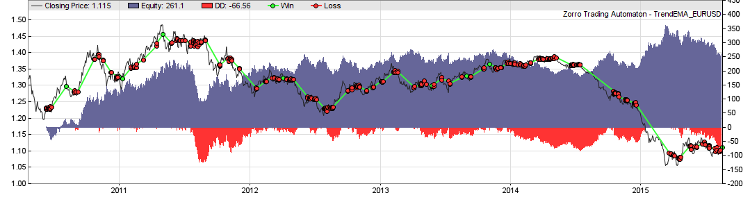
This way the MMI can be an excellent trend filter – in theory. But we all know that there’s often a large gap between theory and practice, especially in algorithmic trading. So I’m now going to test what the Market Meanness Index does to the collection of the 900 trend following systems that I’ve accumulated. For a first quick test, this was the equity curve of one of the systems, TrendEMA, without MMI (44% average annual return):
This is the same system with MMI (55% average annual return):
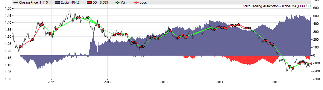
We can see that the profit has doubled, from $250 to $500. The profit factor climbed from 1.2 to 1.8, and the number of trades (green and red lines) is noticeable reduced. On the other hand, the equity curve started with a drawdown that wasn’t there with the original system. So MMI obviously does not improve all trades. And this was just a randomly selected system. If our assumption about trend trendiness is true, the indicator should have a significant effect also on the other 899 systems.
This experiment will be the topic of the next article, in about a week. As usually I’ll include all the source code for anyone to reproduce it. Will the MMI miserably fail? Or improve only a few systems, but worsen others? Or will it light up the way to the Holy Grail of trend strategies? Let the market be the judge.
Next: Testing the Market Meanness Index
Addendum (2022). I thought my above proof of the 3/4 rule was trivial and no math required, but judging from some comments, it is not so. The rule appears a bit counter-intuitive at first glance. Some comments also confuse a random walk (for example, prices) with a random sequence (for example, price differences). Maybe I have just bad explained it – in that case, read up the proof anywhere else. I found the two most elaborate proofs of the 3/4 rule, geometrical and analytical, in this book:
(1) Andrew Pole, Statistical Arbitrage, Wiley 2007
And with no reading and no math: Take a dice, roll it 100 times, write down each result, get the median of all, and then count how often a pair reverted to the median.
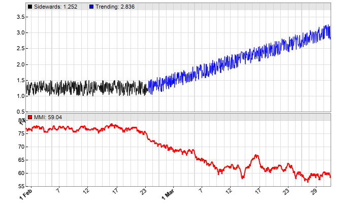
Below you can see the MMI applied to a synthetic price curve, first sidewards (black) and then with added trend (blue). For using the MMI with real prices or price differences, read the next article.
The code:
function run()
{
	BarPeriod = 60;
	MaxBars = 1000;
	LookBack = 500;
	asset(""); // dummy asset
	ColorUp = ColorDn = 0; // don't plot a price curve
	set(PLOTNOW);

	if(Init) seed(1000);
	int TrendStart = LookBack + 0.4*(MaxBars-LookBack);
	vars Signals = series(1 + 0.5*genNoise());
	if(Bar > TrendStart)
		Signals[0] += 0.003*(Bar-TrendStart);
	int Color = RED;
	int TimePeriod = 0.5*LookBack;
	if(Bar < TrendStart)
		plot("Sidewards",Signals,MAIN,BLACK);
	else
		plot("Trending",Signals,MAIN,BLUE);
	plot("MMI",MMI(Signals,TimePeriod),NEW|LINE,Color);
}
This is a really interesting indicator and makes a lot of sense. I had a go at translating the indicator into Amibroker. Not sure if it’s exactly right but it works reasonably well. You can see it posted here: https://decodingmarkets.com/market-meanness-index-amibroker/
Thanks. Your code looks good to me except for the med[bar]. If I understand AFL right, that’s a past array value, but the median must not change inside the loop. So use med[BarCount], not med[bar].
I made this notebook to generate a random walk and then calculate the MMI on it. I wanted to see how this behaves with a known random walk, before I start testing on real assets. Maybe this will be helpful to someone.
https://colab.research.google.com/drive/1n94z1ZFGhBneAGqtefC6OZ1L2xYRC3Ia?usp=sharing
Just wanted to say that I absolutely love it. MMI is the backbone of my algo.
I think your proof is wrong.
I have some ideas of the mistakes in the proof, but it’s kind of obvious that the conclusion is wrong even if you don’t know why. Obviously you don’t have more then 50% in predicting tomorrow in random.
Now to the proof, I think there are atleast two mistakes, one is that the median is not known till the pt day, but more importantly, if pt is the following day to py than the groups are not of same size. The group with one point above m and one below m will be smaller than the other two groups.
Thank you for your comment. You can read up the proof in many statistics books – I did not invent it – but your “median” concept looks wrong. A median of a data sample is simply the 50% divide. It has nothing to do with “past or present days”, and is always known since you know all data values of the sample. If something else is unclear, just ask.
If you want to learn more about the 75% rule and its use in Finance, read “Statistical Arbitrage” by Andrew Pole. He explains the rule on many pages with several proofs.
this is just the classic academic stereotype that love intellectual masturbation rather than application or result.
^ my comment referring back to the discussion back in 2020 with the “masters degree” guy. MMI is just fantastic. thanks for sharing
jcb I read through your conversation with “lurker” and tried their code and it looks right to me. Why would we use MMI when we can just use serial correlation and why would we use if random walks just give the same MMI as trend?
I can at least answer the second part of your question: A purely random walk has serial correlation, and a trending time series has even more serial correlation due to the trend. The purpose of the MMI is differentiating between the two. As to the first part, since the MMI is a measure of serial correlation, you’re in fact using it when using the MMI -if that was the question.
Ok thank you but I just try calculate the MMI of a random walk with trend and random walk without trend and the MMI the same for both. Why are they not different?
I can’t tell since I can’t see your code from here.
Please excuse but I think there is some confusion. That is random noise v random noise with trend. Random walk looks completely different:
https://www.wolfram.com/language/gallery/plot-a-random-walk/
Can you please show random walk v random walk with trend and show MMI go down?
Thank you very much jcb and please excuse if I’m not clear but I think there’s two problems.
Main problem is you are using median for entire price series to calculate MMI and so it look like it go down a little. But in reality we don’t know median of whole price series. On Feb 12 when trend start, as traders we don’t know trend is about to start. At that time we only know median of series up to Feb 12, not median of series including Feb 13, Feb 14 etc. I think this what Sharon mean when she try to talk about lookahead bias. So we have to use rolling median over some span of time from Feb 12 back to some day like Feb 1 or something. If we do that the MMI quickly show no signal for random walk without trend v random walk with trend. I have code below which show.
Second problem even in your example we see MMI barely change. It is at 52 when you start the Trend part on Feb 12 and drop to 50 on Feb 19 then drop to 48 on Feb 22 then back up to 50 on Feb 23 then down to 46 on Feb 26 then at 49 on Mar 2. So I dont see how we can use this to tell when random stock price movements about to turn into a trend.
Code:
import matplotlib.pyplot as plt
import numpy as np
import pandas as pd
def MMI(series):
nh = 0
nl = 0
for i in range(1, len(series)):
m = np.median(series.iloc[:i])
if series.iloc[i-1] > m and series.iloc[i] series.iloc[i-1]:
nh += 1
return 100 * (nh + nl) / len(series)
def MMI_ma(series, timesteps):
series = series.dropna()
list_of_lists = [series.iloc[x[0]:x[1]] for x in zip(range(len(series) – timesteps + 1), range(timesteps, len(series) + 1))]
idx = series.index[timesteps-1:]
ma = pd.Series([MMI(x) for x in list_of_lists], index = idx)
return ma
np.random.seed(16)
diffs_no_trend = np.random.normal(size = 1000)
diffs_with_trend = np.random.normal(size = 1000) + np.ones(shape = 1000) / 4
rwalk_no_trend = np.cumsum(diffs_no_trend)
rwalk_with_trend = np.cumsum(diffs_with_trend)
complete_series = pd.Series(np.concatenate([rwalk_no_trend, rwalk_with_trend]))
plt.figure(figsize=(10,2))
plt.plot(complete_series)
plt.show()
running_MMI = MMI_ma(complete_series, 100)
plt.figure(figsize=(10,2))
plt.plot(running_MMI)
plt.show()
Indeed. There is no “median of whole price series”. A median is always from a sample and is only valid for that sample. And since you now found out that we cannot have the median of tomorrow’s prices, you know the sad truth of finance: the future is unknown. All indicators, including the MMI, use past prices. If I knew the median of tomorrow’s prices, I’d be billionaire and would need no MMI anymore.
The MMI is quite sensitive, as you see from its reaction on regime change in the charts. This is not ‘barely’, but dramatic, at least for a statistical indicator. For its practical use, check out the examples in the subsequent articles. The MMI is meanwhile long established and is one of the most frequent indicators that we use for market change detection. If you haven’t noticed: This article was from 2015.
How can it be useful if its showing 50 when there’s a random walk and then shows 50 again later during when the trend is supposed to be happening?
Price changes are no random walk, they are random noise and have 75% MMI. In practical use you’re not checking a fixed value, but the MMI direction. Normally after lowpass filtering to remove random fluctuations. Look in the code examples. 20% improvement is, at least in finance, normally considered useful. Does this answer your question?
We discovered this site at our fund a few days back, and a number of us have been obsessively reading through the comments with bemused fascination (and some amusement). I wanted to throw in my two cents to try to clear up some of the confusion that seems to be prevalent.
1. The author seems not to understand that there is a difference between random noise and random walks. This is evident by the graphs they keep displaying.
2. The author therefore thinks that the (correct) proof about distribution around the median in random noise can be extrapolated to random walks. It can’t. After all… what is the “median” of a random walk?
3. Several commenters have pointed out this flaw to the author and tried to explain that, since no median exists for the price series as a whole, a median from some arbitrary finite time window in the past of the price series needs to be used, at which point the MMI becomes completely useless, as has been repeatedly demonstrated.
4. I am not aware of any StatArb professionals who use the MMI in their calculations.
5. The book by Andrew Pole that the author seems to revere, “Statistical Arbitrage: Algorithmic Trading Insights and Techniques” is regarded as something of a laughing stock among StatArb guys, and you can even see why in the caustic reviews of the book on Amazon: https://www.amazon.co.uk/Statistical-Arbitrage-Algorithmic-Insights-Techniques/dp/0470138440
For some reason, this article seems to still evoke heavy emotions in some readers, even after almost a decade of MMI usage in hundreds of live strategies. I take this as a compliment. And share amusement about certain comments. But without now again explaining what a random walk is and how a median is calculated – which you can easily read that up in Wikipedia – just out of curiosity: who is “we”?
As someone already mentioned with an example, a perfect trend gives a MMI value of 50%.
In the book (3rd edition, p. 78) you write: “At 100%, any price movement would be compensated immediately by a counter-movement, and at 0% a trend would continue indefinitely”.
One example where I could obtain a value close to 0% was a series consisting of [100, 100,…., 100, 102, 102…, 102] which “feels” less trendy than y=x with 50%.
A series with a value of 100% would be alternating 100, 102, 100, 102… which makes perfect sense.
How would you interpret an MMI of 60% vs one of 45%? Does a lower value mean a longer-term trend is likely to start? Or checking the rate of change in decreasing MMI values would be more appropriate?
“””
How would you interpret an MMI of 60% vs one of 45%? Does a lower value mean a longer-term trend is likely to start? Or checking the rate of change in decreasing MMI values would be more appropriate?
“””
Just to clarify: assumption is we have a peak/valley forming in the low pass filter series as well.
We found that evaluating the MMI slope works normally better for trend regime detection than its absolute value.
You are incorporating lookahead bias in the code for your MMI function (which I have reposted below). Look at the line which says “double m = Median(Data,Length);”. Imagine you set Length = 50, then you will get the median of the series Data[0] to Data[49] (inclusive). But you have specified that Data[0] is the newest data point. So when, in the for loop, you loop through from Data[1] to Data [49], checking if each one is greater than the median and greater than the previous data point, you are making reference to a median that hasn’t happened yet. How can Data[1] check whether it’s greater or less than a median which incorporates Data[0] into its calculation? Data[0] is the newest data point, and so happens *after* Data[1], meaning that Data[1] cannot compare itself to it (as Data[0] is in the future from the perspective of Data[1]). Likewise, Data[1] happens *after* Data[2], and so Data[2] cannot compare itself to any median which incorporates data from Data[1] or Data[0]. Etc etc. By the time you’ve gotten all the way back to Data[49], it’s comparing itself to a median which is incorporating data from 48 days in the future from its perspective.
Do you know what the median of the S&P500 is going to be over the next 48 days? Because that’s the sort of information you’d need to use this thing in the real world like how you’re using it in your tests. In reality, each data point could only compare itself to the median of the data points which were before it in time. So if you specified Length=50, what should happen is that Data[0] would compare itself to the median of Data[1] to Data[50] (inclusive), Data[1] would compare itself to the median of Data[2] to Data[51] (inclusive), Data[2] would compare itself to the median of Data[3] to Data[52] (inclusive), etc. This is doubtless why you’re getting so many spurious successes with this algorithm in your tests.
double MMI(double *Data,int Length)
{
double m = Median(Data,Length);
int i, nh=0, nl=0;
for(i=1; i m && Data[i] > Data[i-1]) // mind Data order: Data[0] is newest!
nl++;
else if(Data[i] < m && Data[i] < Data[i-1])
nh++;
}
return 100.*(nl+nh)/(Length-1);
}
Data series go from newest to oldest data and don’t extend into the future. That’s why no indicator based on such a series can have “lookahead bias”, unless you intentionally add future data.
The median of the S&P500 isn’t the same as it was 100 days ago, and that isn’t the same as it was 500 days ago, or 1000 days ago or 5000 days ago. The S&P500 has no static median for you to compare your data points with. Neither does the FTSE100, Google’s stock price, Apple’s stock price or any other price series. So you can only calculate the median with respect to some finite time window, and then use the MMI to compare your data points to that.
So if you’re calculating the MMI for today, your median needs to be calculated based on data points going from yesterday up to some number of days in the past (e.g. 50 days), because that median isn’t going to have the same value in future. You don’t know what the data points will be tomorrow, the day after that, etc, so you can’t incorporate them into your calculation of the median when you try and calculate the MMI today. That’s what’s wrong with your code. Each day in your for loop is comparing itself to a median which incorporates future data points (from that day’s perspective), and so is subject to lookahead bias.
For anything that you calculate, like MMI or median, you can only use past data points. You cannot use future data, because you simply don’t have it in your data series. This has nothing to do with the MMI, but is valid for any time series based indicator. So what exactly is the problem?
Because in your code, one of the things you’re doing is calculating the number of data points over the last N days which are above or below the median… of the last N days. So if the MMI shows that the sequence of N-1 data points is trending, that means it’s trending with respect to a median that hasn’t even happened yet. That median can’t be calculated until the Nth day in the lookback window. So if you had been sitting at your desk in the office 10 days ago, it’s no good saying your stock was trending with respect to the median calculated from *today* over a 15 day lookback period. Because today hadn’t happened yet for you. Neither had the other 9 days that lay between then and now. The only thing you’d have to go on, sitting there in your office 10 days ago, is the data that was available at the time. I.e. a median calculated from data that was older than 10 days ago.
Since you always use data from the past, you cannot have “trend with respect to a future median”. You can only have trend that developed during the past N days.
If you knew a future median, you needed no MMI – you’d be billionaire anyway. And anyone else too, money would lose any value, civilization would collapse. So you should be glad that the future is unknown. 🙂
Your method of determining whether a trend exists is by comparing the data points to a median. If the median changes, the values of nl and nh will change, your MMI will change, and your conclusion as to whether you’re observing a trend will change. So the trend is with respect to a median. A median that your code is looking ahead to calculate. If you engaged with criticism that is levelled against your code rather than just dismissing it you might be able to make it better.
I welcome criticism, but it should make at least a bit of sense. Your first comment did, you simply got the time series direction wrong. I hope I could help you with that. But now you’ve lost me. What code is “looking ahead”? How can you look ahead when using only past data? Look ahead to what? Please explain.
It is the easiest thing in the world to lookahead with past data. If you are unfamiliar with the concept of lookahead bias, this video explains it quite well:
https://m.youtube.com/watch?v=cCdVcbdtkSk
If it helps, let’s consider a simpler example. Forget the MMI, our trading strategy is the following:
1. Calculate the median M from Day[0] back to Day[49]
2. For i = 1 to 49, calculate Delta = Day[i]-M. If Delta 0 sell the asset.
3. Rinse and repeat. You’ll be a millionaire in no time… according to your backtest at least.
If Delta is greater than 0 sell the asset. If Delta is less than 0 buy the asset. *
Don’t know why certain characters are getting cut out in my comments.
🙂 🙂 🙂 I will certainly congratulate you to your upcomming billions – only please reveal which one of your 49 Deltas you will pick for that buying or selling at Day[0].
If you assumed you could trade the Delta on any day: it’s not so since neither your median nor any of your Deltas are available before day[0]. From time to time I see people coming up with ingenious systems that make them billionaire but miss 2 tiny details: a) the future is unknown b) the past can’t be altered.
I suspect you will find in your code that you are doing something akin to that, thereby accounting for the high degree of success of the algorithm in backtests. We know that the MMI can’t distinguish trends from random walks because as others have highlighted it gives a score of 50% for a trend and a score of 50% for a random walk, so this is the only way to account for its success in backtests (I know you have struggled to understand that there is a difference between random walks from random noise in the past with other commentators, so I will leave that discussion alone and just leave it to you to read up on the two things).
Since the code uses nowhere any future data, I’m not sure where you see future peeking. Anyway, if you feel that you will find something in my code, you’re always welcome to share your feelings with the world. Until you found that something, I consider this issue solved and your question answered.
Hi there to all, for the reason that I am genuinely keen of reading this website’s post to be updated on a regular basis. It carries pleasant stuff.
A Forex prop calculator helps traders plan risk, position size, and profit targets with precision while trading a funded firm account. It gives accurate insights into lot size, leverage, and drawdown limits, helping traders follow rules, stay disciplined, and maximize performance in professional Forex prop trading environments.
Teknolojiye çok hakim olmayanlar için başlangıçta karışık gelebilir.