
We can see thinking machines taking over more and more human tasks, such as car driving, Go playing, or financial trading. But sometimes it’s the other way around: humans take over jobs supposedly assigned to thinking machines. Such a job is commonly referred to as a Mechanical Turk in reminiscence to Kempelen’s famous chess machine from 1768. In our case, a Mechanical Turk is an automated trading algorithm based on human intelligence.
Theoretically, many trend trading systems would fall in the Turk category since they are based on following the herd. But here we’re not looking into trader’s opinions of the current market situation, but into their expectations of the future. There are several methods. The most usual is evaluating the Commitment Of Traders report, for which many platforms, also Zorro, provide easy-to-use indicators. But some publications (1) found that using the COT report for predicting the markets produces mixed results at best.
There’s a more precise way to get the market’s expectations. It’s using options premiums. If an option expires in 6 weeks, its current premium reflects what option buyers or sellers think about the underlying price in 6 weeks.
The price probability distribution
For deriving the expected underlying price at expiration, we have to take all strike prices in consideration. Here’s the algorithm in short (I haven’t invented it, a longer description can be found in (2)). Assume SPY is currently trading at $200. For getting the probability that it will rise to between 210 and 220 in 6 weeks, we’re looking into the 210 call and the 220 call. Suppose they trade at $14 and $10. So we can buy the 210 call and sell the 220 call and pay $4 difference. If at expiration SPY is under 210, both contracts have no worth and we lose the 4 dollars. If it is above 220, our gain is the $10 strike difference minus $4 premium difference, so we win 6 dollars. If it is between 210 and 220, our win or loss is also inbetween, with an average of (-4+6)/2 = 1 dollar.
When options prices are “fair”, i.e. solely determined by probabilities where the price will end up at expiration, summing up over all possible outcomes yields zero profit or loss. So
-$4×L + $1×M + $6×H = $0
where L is the probability for SPY to end up below 210, M is the probability that it will be between 210 and 220, and H is the probability that it will be above 220. Since one of these three alternatives will always happen, the sum of all 3 probabilities must be 1:
L + M + H = 1
Now let’s assume that we know L already. Then we have two equations with two unknowns, which are easily solved:
5L – 5H = 1 => H = L – 0.2
10L + 5M = 6 => M = 1.2 -2L
Assuming L = 50% yields H = 30% and M = 20%.
How do we now get the value L? We simply take the lowest strike offered at the market, and assume that the probability of SPY ending up even below that is zero. So our first L is 0. We can now use the method above to calculate the M belonging to the interval between the lowest and the second-lowest strike. That M is then added to L since it’s the probability of SPY ending up at or below the second-lowest strike. We continue that process with the next interval, getting a specific L and M for any interval until we arrived at the highest strike. If the traders have been consistent with their assumptions, the final L – the sum over all Ms – should be now at or close to 1.
Here’s a small script that displays the 6-weeks L distribution of SPY:
void main()
{
	StartDate = 20170601;
	LookBack = 0;

	assetList("AssetsIB");
	asset("SPY");

// load today's contract chain
	contractUpdate(0,0,CALL|PUT);
	printf("\n%i contracts",NumContracts);
	if(!NumContracts) return;

// get underlying price
	var Price,Current = priceClose(0);
	printf("\nCurrent price %.2f",Current);

// plot CPD histogram
	contractCPD(45);	// 6 weeks
	int N = 0;
	for(Price = 0.75*Current; Price < 1.25*Current; N++, Price += 0.01*Current)
		plotBar("CPD",N,floor(Price),cpd(Price),BARS|LBL2,RED);
	printf("\nExpected price %.2f",cpdv(50));

// compare with real future price
	set(PEEK);
	N = timeOffset(UTC,-45,0,0);
	printf("\nFuture price %.2f",priceClose(N));
}
The result is a histogram of expected probabilities, in percent, that the SPY price will be at or below the price at the x-axis six weeks in the future. I’ve marked the current price with a black bar.
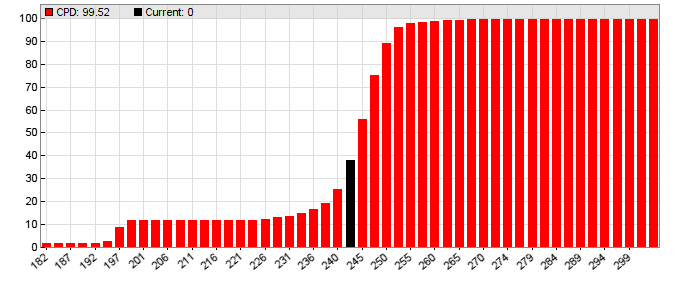
The contractCPD function generates the distribution with the above described algorithm, cpd returns the accumulated probability L (in percent) at a given price, and cpdv returns the price at a given L. Therefore, cpdv(50) is the median of market expectations. In our case, at June 1 2017, a modest price increase to $245 was expected for mid-July (in fact the price ended up at $245.51, but don’t get too excited – often trader’s expectations fall short by several dollars). We can also see an unusal step at the begin of the histogram: about 10% of traders expected a strong drop to below $200. Maybe Trump twittered something that morning.
The strategy
We will now exploit trader’s expectations for a strategy, and this way check if they have any merit. This is our mechanical Turk:
#define Sentiment AssetVar[0]

void run()
{
	StartDate = 20120102;
	EndDate = 20171231;
	BarPeriod = 1440;

	assetList("AssetsIB");
	asset("SPY");
	MaxLong = MaxShort = 1;

// load today's contract chain
	contractUpdate(0,0,CALL|PUT);
	int N = contractCPD(45);

// increase/decrease market sentiment
	if(N) {
		var Expect = cpdv(50) - priceClose();
		if(Expect < 0)
			Sentiment = min(Expect,Sentiment+Expect);
		else
			Sentiment = max(Expect,Sentiment+Expect);
	}
	if(Sentiment > 5)
		enterLong();
	else if(Sentiment < -5)
		enterShort();

	plot("Sentiment",Sentiment,NEW,RED);
}
We’re checking the market expectation every day and add it to a previously defined Sentiment asset variable. If the expectation changes sign, so does Sentiment. If its amount has accumulated above 5, we buy a long or short position dependent on its sign. This way we’re only considering the market expectation when it’s either relatively strong or had the same direction for several days.
The result:
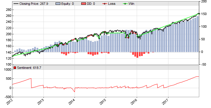
The system produces about 20% annual return with profit factor 3. The red line in the lower chart is the Sentiment variable – we can see that it often steadily increases, but sometimes also decreases. Since SPY normally rises, shorting it with this strategy produces less profit than going long, but is still slightly profitable with an 1.16 profit factor.
Predicting the price in 6 weeks
What are traders currently thinking of the SPY price in 6 weeks? For this, the first script above needs just be slightly modified so that it does not use historical options data, but connects to IB and downloads the current options chain with all prices:
void main()
{
	StartDate = NOW;
	LookBack = 0;

	assetList("AssetsIB");
	asset("SPY");

// load today's contract chain
	contractUpdate(0,0,CALL|PUT);
	printf("\n%i contracts",NumContracts);
	if(!NumContracts) return;

// get underlying price
	var Price,Current = priceClose(0);
	printf("\nCurrent price %.2f",Current);

// plot CPD histogram
	printf("\nWait time approx %i minutes",1+NumContracts/200);
	contractCPD(45);
	int N = 0;
	for(Price = 0.75*Current; Price < 1.25*Current; N++, Price += 0.01*Current)
		plotBar("CPD",N,floor(Price),cpd(Price),BARS|LBL2,RED);
	printf("\nExpected price %.2f",cpdv(50));
}
This script must be started in Zorro’s Trade mode with the IB plugin selected. Mind the displayed “wait time”. IB sometimes needs up to ten seconds for returning the price of an option contract, so downloading the prices of all 6-weeks contracts can take half an hour or more.
I ran that script today (Dec 11 2018) and the option traders expect the SPY price to rise to $269 in six weeks. So I’ll check the price by the end of January and post here if they have been right.
I’ve added the scripts to the 218 repository. You’ll need Zorro 1.99 or above, and SPY options EOD history for the first 2 scripts. You’ll really have to buy it this time, the free artificial options history won’t do for market sentiment.
Conclusions
- A Turk can beat a thinking machine.
- Option traders tend to underestimate future price changes.
- But they are often right in the price direction.
Literature
(1) Sanders, Irwin, Merrin: Smart Money? The Forecasting Ability of CFTC Large Traders (2007)
(2) Pat Neal, Option Prices Imply a Probability Distribution
Great to have you back! I was missing your articles. Zorro is a beauty! Thank you. Are you on twitter?
Excellent and innovative approach!
What would you suggest investigating as the lowest cost way to build SPY option price history to test your strategy?
Thanks
Thank you. No, I’m not on Twitter, and for options price history we normally recommend iVolatility to clients.
Thank you so very much for sharing your knowledge with us. Thank you also for the fantastic work on Zorro! It’s absolutely marvelous to see you back…
Hello, very nice article as usual.
I’d like to share with you a doubt about this approach: the formula assumes the prices are “fair”, which might not be and this I believe can lead to a misbehaviour. Sticking to your example, the line “M = 1.2 -2L”, could lead to a negative M if L > 60% when the calculation algorithm gets to those 2 calls. I’ve taken an option chain from yahoo, put it in a spreadsheet and implemented the formulas explained in the article, and I get negative M here and there. How does contractCPD handle this? I can’t quite figure out a clever solution, I thought we could try to use a “starting L” > 0 so that no negative Ms occur, but there’s no such value in the chain I got.
Thanks,
Simone
Yes, since many effects influence option prices, the model is a bit simplistic. Some option buyers do not speculate on future prices at all, but buy options for insurance, and this way distort the price distribution. So the price distribution is no guarantee to reflect the real probabilities. The contractCPD function is more complex than described here, f.i. it calculates the probabilities from both ends at L=0 and L=1, and also uses an algorithm for fixing gaps or negative probabilities.
Thank you, I expected using both ends was likely to be the improvement for that.
Simone, would You like to share your file?
Not sure what I am doing wrong, but I am getting a crash in what looks like the contractCPD function:
Load AssetsIB
!SPY: 272.77000 0.03000 1
SPY: 0..8765
!Get Option Chain SPY-OPT–0–SMART–USD
Chain of 3243 SPY contracts
3243 contracts today
Current price 272.77
Wait time approx 17 minutes
Error 111: Crash in function: main() at bar 0
Logout.. ok
I don’t know either, but places where you can get help with coding or crashes are the Zorro forum or Zorro support.
JCL, doesn’t a simple BUY and HOLD strategy beat this?
Wouldn’t that be boring?
Haha! Good point!
But when testing the strategy script above with the SPY.t8 data provided on Zorro’s site, the trades don’t match up. It would be nice to reproduce the results in your blog. Any ideas?
The reason is different history. Theoretically, option history should not depend on the vendor. The backtest with the above equity curve was with option history from IVolatility. The option data on the download page is from a different source, for cost reasons. The data is almost identical, but not quite. This has normally no effect on the backtest, but in this case it leads to slightly different trades.
For future blog articles I’ll use the data from the Zorro download page.
Hi, <3
When Linux port?
When buying Zorro S and The BlackBook with Bitcoins?
Despite copying and pasting the code into Zorro 2.15, “Expect” is always positive for me and “Sentiment” is just a straight line with a positive slope. As a result, the algo doesn’t generate slightly different trades but a single buy-and-hold trade for the length of the backtest. I’m using the SPY options data from the Zorro website and an SPY price history downloaded from Yahoo.
You need not copy and paste. The “Turk” script is included in Zorro 2.15. However, it’s of course no “trading system” and its backtest return will depend on the test period.
FYI option contracts do not reflect the future price of an asset but the future level of volatility of this asset, futures contract do. There is a biais in your analysis as out of the money options tend to be over paid as they represent a great hedge against large movements of the market, especially put options against market crashes. The existence of smile of volatility proves this fact. Also, large financial institutions do not use option in directional strategies on the price of the underlying asset but on the anticipation of the future fluctuations. To make it simple, these strategies are delta flat and long gamma (long options) when the market goes down as the risk anticipation increases and short gamma during up trends (short options) as the level of risk anticipation and thus volatility decreases and so do the options prices. Another large trading activity is called the delta one in which options are used to replicate the underlying for instance by buying a call and selling a put of same strike ( for the long strategy), the objective being speculating on the dividend. Your demonstration is truly interesting on the mathematical point of view but unfortunately options prices are not fair at all, and indeed as someone noticed, a simple buy and hold would perform better on the SPY.
Hi Jordan,
Are you JCL from JCLs Forex group? The domain was jclcapital.com?
Regards,
Gavin
Afraid I’m neither Jordan, nor from jclcapital.com. Seems they have stolen my initials.
Hi jcl,
In the black book and zorro trader manual there are examples of training parameters optimization
where graphs contains PRR results and then “plateau” is selected. How PRR is calculated per subset ? Are they aggregated by parameter value and then mean is taken, does optimizator is doing any filtering ?
Does ascent optimization in zorro trader platform based on any open-sourced algorithm ?
If you are interested in any suggestions, it would be really interesting to see post about training parameter optimization in future.
Best Regards,
Eugene
Zorro calculates the training objective with a user supplied “objective” function. If none is supplied, a default function is used that returns the PRR. You can find this function in the “default.c” code. I believe the Ascent algorithm is not open source.
Thank you jcl for reply.
What I meant if you have training params(fastN,slowN,stoploss) [ 1 2 3] with prr 1 and [ 1 2 4] with prr 2. So for the parameter fastN with value 1 would have PRR 1.5 ?
Suppose PRR 1.5 is the highest “mean” PRR and near by values of fastN are also high. Then, fastN with value 1 would be considered as best ?
This is based on the documentation “Evaluates the effect of any parameter on the strategy separately.”
In your example, [1 2 3] => PRR 1 and [1 2 4] => PRR 2, the parameters fastN,slowN can have no PRR at all because their effect on the strategy is unknown. Only stoploss can be determined with a PRR gradient of 1. At least that would be my interpretation of determining the effect of a parameter.
Hi JCL,
I have tried the code but on 1 week or even 3 days of expiration, in real, on SPY, AMZN, TLT, TSLA, etc. On such short DTE, it does not provide better results than 52%. I think that it is because the number of days are too small and the numbers not statistically significant. Is that correct? 6 weeks of DTE would work better?
Yes, the DTE is a compromise between significance of the effect and timeliness of the prediction.
Hi JCL,
I think there is an error while deriving the equations. 5L – 5H = 1 leads to H=L-0.2, not H=0.2+0.2L. Has this an influence on the article?
Indeed. Apparently you’re the first one who checked that equation.
I’ve corrected the article. The end result H = 30% is correct, though. I had probably copied a wrong line from my scrap paper.
Hi JCL,
when running the script predicting the price in 6 weeks, it connects correctly to my IB, but then gives me back the error : “Error 111 crash in main : main()”. Do you know how I can fix this issue? Zorro version is 2.30.
2.30 was a very old version, but should work with this script. Even if not, there is no line in the script that would cause a crash. I suspect a more serious reason, like a corrupted installation. Get a recent Zorro, install it, and run the script again. The current version is 2.44. Run also a malware check on that PC, just to be on the safe side.
Hi JCL,
sorry for my previous post, it is useless. After installing new version of Zorro all is working perfectly. I should have checked before posting… By the way, your article is very interesting and novative. Should this methode be working for shorter periods, like 14 days?
It is less effective in short periods because the predicted price is then too close to the current price. But I did not run very extensive tests – maybe you can find a way to make it work on short periods.
Yes, I am actually making tests in real on different time intervals and different symbols. I will publish the results here.
Hi JCL,
is there an equivalent native Python function for contractCPD() function?
I know none. But it should not be too difficult to program one with the above algorithm.
Hi jcl,
I tried to run the Turk2 script present in the version of Zorro S 2.50 but I get absurd results .. do you have any idea?
Test Turk2 SPY, Zorro 2.502
Simulated account AssetsIB (NFA)
Bar period 24 hours (avg 2091 min)
Total processed 2617 bars
Test period 2012-01-05..2019-03-01 (1798 bars)
Lookback period 0 bars (0 minutes)
Montecarlo cycles 200
Simulation mode Realistic
Spread 2.0 pips (roll 0.00/0.00)
Commission 0.01
Lot size 1.00
Gross win/loss 21.62$-0$, +2161.9p, lr 8.53$
Average profit 3.02$/year, 0.25$/month, 0.0116$/day
Max drawdown -0.37$ 1.7% (MAE -13.75$ 63.6%)
Total down time 0% (TAE 12%)
Max down time 34 hours from Jan 2012
Max open margin 64.02$
Max open risk 1.31$
Trade volume 128$ (17.91$/year)
Transaction costs -0.0200$ spr, -0.0053$ slp, 0$ rol, -0.0100$ com
Capital required 64.26$
Number of trades 1 (1/year)
Percent winning 100.0%
Max win/loss 21.62$ / -0$
Avg trade profit 21.62$ 2161.9p (+2161.9p / -0.0p)
Avg trade slippage -0.0053$ -0.5p (+0.0p / -0.0p)
Avg trade bars 268 (+268 / -0)
Max trade bars 268 (77 weeks)
Time in market 15%
Max open trades 1
Max loss streak 0 (uncorrelated 0)
Annual return 5%
Reward/Risk ratio 58.8
Sharpe ratio 0.45 (Sortino 0.47)
Kelly criterion 4.37
Annualized StdDev 10.39%
R2 coefficient 0.000
Ulcer index 22.9%
Scholz tax 6 EUR
Year Jan Feb Mar Apr May Jun Jul Aug Sep Oct Nov Dec Total
2012 5 9 6 -1 -13 7 3 5 4 -4 1 0 +22
2013 11 0 0 0 0 0 0 0 0 0 0 0 +11
2014 0 0 0 0 0 0 0 0 0 0 0 0 +0
2015 0 0 0 0 0 0 0 0 0 0 0 0 +0
2016 0 0 0 0 0 0 0 0 0 0 0 0 +0
2017 0 0 0 0 0 0 0 0 0 0 0 0 +0
2018 0 0 0 0 0 0 0 0 0 0 0 0 +0
2019 0 0 0 +0
Confidence level AR DDMax Capital
10% 5% 0 64.24$
20% 5% 0 64.25$
30% 5% 0 64.26$
40% 5% 0 64.27$
50% 5% 0 64.28$
60% 5% 0 64.30$
70% 5% 0 64.32$
80% 5% 1 64.36$
90% 5% 1 64.42$
95% 5% 1 64.47$
100% 5% 1 64.58$
Portfolio analysis OptF ProF Win/Loss Wgt%
SPY:L .1000 ++++ 1/0 100.0
You’re probably using multiple SPY option history files, not a single file history as in the original code. In that case you must give the asset name, or ‘Asset’, in the contractUpdate call.
contractUpdate(Asset,0,CALL|PUT);
Otherwise Zorro only uses the already loaded data and that’s only one year.
Hi jcl,
strange but when I try to generalize your equations within a Python code like this :
# Equation parameters
alpha = price_high – price_low # Premiums
DStr = strike_high – strike_low # Strikes
a = (2*alpha+DStr)/2
b=DStr + alpha
if L==0 :
M = b/(b-a)
L = M
else:
M = b/(b-a)*(1+L*(alpha-b)/b)
L = L + M
I get negative values or bigger than 1 values for L. Unless I am wrong in my generalized equations, do you see an error?
Here is what I get for SPY, DTE = 2025-01-17:
Probability for each strike interval:
Between 180.0 and 185.0: Probability = -1.3440
Between 185.0 and 190.0: Probability = -17.1920
Between 190.0 and 195.0: Probability = 33.0880
Between 195.0 and 200.0: Probability = -34.0520
Between 200.0 and 205.0: Probability = 32.6920
Between 205.0 and 210.0: Probability = -51.5360
Between 210.0 and 215.0: Probability = 64.6440
Between 215.0 and 220.0: Probability = -83.1360
Between 220, etc.