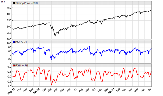
John Ehlers strikes again. The TASC January 2022 issue features another indicator supposedly improved with Hann windowing – the RSIH, a RSI with Hann flavour. Can it beat the standard RSI?
The RSI is basically the normalized difference of price up/down movements. And its here presented Hann variant filters the price differences with a Hann window that was described in a previous article on this blog. The RSIH code in C for Zorro is not very complex:
var RSIH(vars Data, int Length)
{
  var CU = 0, CD = 0;
  int i;
  for(i=1; i<Length; i++) {
    var D = Data[i-1]-Data[i];
    var Hann = 1-cos(2*PI*i/(Length+1));
    if(D > 0) CU += Hann*D;
    else if(D < 0) CD -= Hann*D;
  }
  if(CU+CD != 0)
    return (CU-CD) / (CU+CD);
  else return 0;
}
According to Ehlers, the optimal Length parameter is the dominant cycle of the price series. Here’s the RSIH (red) applied to a SPY chart, in comparison with a standard RSI (blue):

Indeed the RSIH curve looks a lot smoother and better to trade than the original RSI curve. But the usual question for any new indicator is “What can I do with it?” and as usual the indicator inventor remains silent about that. I can only say what you cannot do: replacing the RSI in a working strategy with RSIH. Even when adapting the scale and thresholds, in all RSI based strategies that I tested the RSIH produced a worse result. Maybe John Ehlers gives a practical example in a future article.
The RSIH indicator and test script can be downloaded from the 2021 script repository.

> I can only say what you cannot do: replacing the RSI in a working strategy with RSIH.
Not much luck here either.
Somehow I find RSIS most useful although not a huge fan of RSI concept to begin with.
And still failing to find a use for windowing.
Adding a windowing function to an indicator smooths the output, but at the cost of additional phase delay (lag). Window functions, such as Hann, Hamming, and Blackman, are effectively low pass finite impulse response (FIR) filters, which, like all low pass filters, result in the smoothing. The longer the window length, the more the smoothing, but also the more the phase delay, an unavoidable tradeoff. So, while the additional smoothing can help avoid some of the whipsaws, the added delay also slows the response to rapid changes in longer-term trends, which most likely is responsible for the worsened performance. The smoothed windowed output looks nice on a chart, though!
Thanks for this interesting and very useful blog.
The Hann Function to generate an array of smoothing coefficients is widely published and implemented, eg;
Matlab https://uk.mathworks.com/help/signal/ref/hann.html
Scipy https://docs.scipy.org/doc/scipy/reference/generated/scipy.signal.windows.hann.html
Here’s the formula:
0.5 cos(2πn/(N-1))
N = length of window
However the formula Ehlers uses is different:
1 – cos(2πn/(N+1))
In Python an 8 element, standard Hann Window is :
import numpy as np
N = 8
n = np.arange(N)
0.5 * (1 – np.cos(2*math.pi*(n/(N-1))))
0. , 0.1882551 , 0.61126047, 0.95048443, 0.95048443, 0.61126047, 0.1882551, 0.
(this matches the output from the Matlab and Scipy implementations)
If we use Ehlers formula, again in Python, the output is quite different
N=8
X = np.arange(1, N+1)
1 – np.cos(2*math.pi*(n/(N+1)))
0, 0.23395556, 0.82635182, 1.5, 1.93969262, 1.93969262, 1.5, 0.82635182
So what’s going on here ?
I have read through Ehler’s two articles in TASC (Sep 2021 and Jan 2022), have spent several hours coding away and feel none the wiser!
Now I realise there are two ways to calculate the Hann coefficients:
Symmetric: 0.5 cos(2πn/(N-1))
Periodic: cos(2πn/(N+1))
“This option is useful for spectral analysis because it enables a windowed signal to have the perfect periodic extension implicit in the discrete Fourier transform.”