Hacking a HFT system

Compared with machine learning or signal processing algorithms of conventional algo trading strategies, High Frequency Trading systems can be surprisingly simple. They need not attempt to predict future prices. They know the future prices already. Or rather, they know the prices that lie in the future for other, slower market participants. Recently we got some contracts for simulating HFT systems in order to determine their potential profit and maximum latency. This article is about testing HFT systems the hacker’s way.

The HFT advantage is receiving price quotes earlier and getting orders filled faster than the majority of market participants. Its profit depends on the system’s latency, the delay between price quote and subsequent order execution at the exchange. Latency is the most relevant factor of a HFT system. It can be optimized in two ways: by minimizing the distance to the exchange, and by maximizing the speed of the trading system. The former is more important than the latter.

The location

Ideally, a HFT server is located directly at the exchange. And indeed most exchanges are dear selling server space in their cellars – the closer to the main network hub, the dearer the space. Electrical signals in a shielded wire travel with about 0.7 .. 0.9 times the speed of light (300 km/ms). 1 m closer to the signal source means a whopping 8 nanoseconds round-trip time advantage. How many trade opportunities disappear after 8 ns? I don’t know, but people are willing to pay for any saved nanosecond.

Unfortunately (or fortunately, from a cost perspective), the HFT system that we’ll examine here can not draw advantage from colocating at the exchange. For reasons that we’ll see soon, it must trade and receive quotes from the NYSE and the CME simultaneously. There’s a high speed cable and also a microwave radio link running between both cities. The theoretically ideal location of such a HFT system is Warren, Ohio, exactly halfway between New York City and Chicago. I don’t know whether there’s a high speed node in Warren, but if it is, the distance of 357 miles to both exchanges would be equivalent to about 4 ms round-trip latency.

Without doubt, a server in this pleasant town would come at lower cost than a server in the cellar of the New York Stock Exchange. My today’s free tip for getting rich: Buy some garage space in Warren, tap into the high speed New York-Chicago cable or radio link, and rent out server racks!

The software

When you’ve already invested money for the optimal location and connection of the HFT system, you’ll also want an algo trading software that matches the required speed. Commercial trading platforms – even Zorro – are normally not fast enough. And you don’t know what they do behind your back. HFT systems are therefore normally not based on a universal trading platform, but directly coded. Not in R or Python, but in a fast language, usually one of the following:

• C or C++. Good combination of high level and high speed. C is easy to read, but very effective and the fastest language of all – almost as fast as machine code.
• Pentium Assembler. Write your algorithm in machine instructions. Faster than even C when the algorithm mostly runs in loops that can be manually optimized. There are specialists for optimizing assembler code. Disadvantage: Any programmer has a hard time to understand assembler programs written by another programmer.
• CUDA, HLSL, or GPU assembler. Run your algorithm on the shader pipeline of the PC’s video card. This makes sense when it is heavily based on vector and matrix operations.
• VHDL. If any software would be too slow and trade success really depends on nanoseconds, the ultimate solution is coding the system in hardware. In VHDL you can define arithmetic units, digital filters, and sequencers on a FPGA (Field Programmable Gate Array) chip with a clock rate up to several 100 MHz. The chip can be directly connected to the network interface.

With exception of VHDL, especially programmers of 3D computer games are normally familar with those high-speed languages. But the standard language of HFT systems is plain C/C++. It is also used in this article.

The trading algorithm

Many HFT systems prey on traders by using fore-running methods. They catch your quote, buy the same asset some microseconds earlier, and sell it to you with a profit. Some exchanges prevent this in the interest of fair play, while other exchanges encourage this in the interest of earning more fees. For this article we won’t use fore-running methods, but simply exploit arbitrage between ES and SPY. We’re assuming that our server is located in Warren, Ohio, and has a high speed connection to Chicago and to New York.

ES is a Chicago traded S&P500 future, exposed to supply and demand. SPY is a New York traded ETF, issued by State Street in Boston and following the S&P500 index (minus State Street’s fees). 1 ES Point is equivalent to 10 SPY cents, so the ES price is about ten times the SPY price. Since both assets are based on the same index, we can expect that their prices are highly correlated. There have been some publications (1) that claim this correlation will break down at low time frames, causing one asset trailing the other. We’ll check if this is true. Any shortlived ES-SPY price difference that exceeds the bid-ask spreads and trading costs constitutes an arbitrage opportunity. Our arbitrage algorithm would work this way:

• Determine the SPY-ES difference.
• Determine its deviation from the mean. 
• If the deviation exceeds the ask-bid spreads plus a threshold, open positions in ES and SPY in opposite directions.
• If the deviation reverses its sign and exceeds the ask-bid spreads plus a smaller threshold, close the positions.

This is the barebone HFT algorithm in C. If you’ve never seen HFT code before, it might look a bit strange:

#define THRESHOLD  0.4  // Entry/Exit threshold 

// HFT arbitrage algorithm
// returns 0 for closing all positions
// returns 1 for opening ES long, SPY short
// returns 2 for opening ES short, SPY long
// returns -1 otherwise
int tradeHFT(double AskSPY,double BidSPY,double AskES,double BidES)
{
	double SpreadSPY = AskSPY-BidSPY, SpreadES = AskES-BidES;
	double Arbitrage = 0.5*(AskSPY+BidSPY-AskES-BidES);

	static double ArbMean = Arbitrage;	
	ArbMean = 0.999*ArbMean + 0.001*Arbitrage;
	static double Deviation = 0;
	Deviation = 0.75*Deviation + 0.25*(Arbitrage - ArbMean);

	static int Position = 0;	
	if(Position == 0) {
		if(Deviation > SpreadSPY+THRESHOLD)
			return Position = 1;
		if(-Deviation > SpreadES+THRESHOLD)
			return Position = 2;
	} else {
		if(Position == 1 && -Deviation > SpreadES+THRESHOLD/2)
			return Position = 0;
		if(Position == 2 && Deviation > SpreadSPY+THRESHOLD/2)
			return Position = 0;
	}
	return -1;	
}

The tradeHFT function is called from some framework – not shown here – that gets the price quotes and sends the trade orders. Parameters are the current best ask and bid prices of ES and SPY from the top of the order book (we assume here that the SPY price is multiplied with 10 so that both assets are on the same scale). The function returns a code that tells the framework whether to open or close opposite positions or to do nothing. The Arbitrage variable is the mid price difference of SPY and ES. Its mean (ArbMean) is filtered by a slow EMA, and the Deviation from the mean is also slightly filtered by a fast EMA to prevent reactions on outlier quotes. The Position variable constitutes a tiny state machine with the 3 states long, short, and nothing. The entry/exit Threshold is here set to 40 cents, equivalent to a bad SPY spread multiplied with 10. This is the only adjustable parameter of the system. If we wanted to really trade it, we had to optimize the threshold using several months’ ES and SPY data.

This minimalistic system would be quite easy to convert to Pentium assembler or even to a FPGA chip. But it is not really necessary: Even compiled with Zorro’s lite-C compiler, the tradeHFT function executes in just about 750 nanoseconds. A strongly optimizing C compiler, like Microsoft VC++,  gets the execution time down to 650 nanoseconds. Since the time span between two ES quotes is normally 10 microseconds or more, the speed of C is largely sufficient.

Our HFT experiment has to answer two questions. First, are those price differences big enough for arbitrage profit? And second, at which maximum latency will the system still work? 

The data

For backtesting a HFT system, normal price data that you can freely download from brokers won’t do. You have to buy high resolution order book or BBO data (Best Bid and Offer) that includes the exchange time stamps. Without knowing the exact time when the price quote was received at the exchange, it is not possible to determine the maximum latency.

Some companies are recording all quotes from all exchanges and are selling this data. Any one has its specific data format, so the first challenge is to convert this to lean data files that we then evaluate with our simulation software. We’re using this very simple target format for price quotes:

typedef struct T1    // single tick
{
	double time; // time stamp, OLE DATE format
	float fVal;  // positive = ask price, negative = bid price	
} T1;

The company watching the Chicago Mercantile Exchange delivers its data in a specific CSV format with many additional fields, of which most we don’t need here (f.i. the trade volume or the quote arrival time). Every day’s quotes are stored in one CSV file. This is the Zorro script for pulling the ES December 2016 contract out of it and converting it to a dataset of T1 price quotes:

//////////////////////////////////////////////////////
// Convert price history from Nanotick BBO to .t1
//////////////////////////////////////////////////////

#define STARTDAY 20161004
#define ENDDAY   20161014

string InName = "History\\CME.%08d-%08d.E.BBO-C.310.ES.csv";  // name of a day file
string OutName = "History\\ES_201610.t1";
string Code = "ESZ";	// December contract symbol

string Format = "2,,%Y%m%d,%H:%M:%S,,,s,,,s,i,,";  // Nanotick csv format
void main()
{
	int N,Row,Record,Records;
	for(N = STARTDAY; N <= ENDDAY; N++)
	{
		string FileName = strf(InName,N,N+1);
		if(!file_date(FileName)) continue;
		Records = dataParse(1,Format,FileName);  // read BBO data
		printf("\n%d rows read",Records);
		dataNew(2,Records,2);  // create T1 dataset
		for(Record = 0,Row = 0; Record < Records; Record++)
		{
			if(!strstr(Code,dataStr(1,Record,1))) continue; // select only records with correct symbol
			T1* t1 = dataStr(2,Row,0);  // store record in T1 format
			float Price = 0.01 * dataInt(1,Record,3);  // price in cents
			if(Price < 1000) continue;  // no valid price
			string AskBid = dataStr(1,Record,2);
			if(AskBid[0] == 'B')  // negative price for Bid
				Price = -Price;
			t1->fVal = Price;
			t1->time = dataVar(1,Record,0) + 1./24.;  // add 1 hour Chicago-NY time difference
			Row++;
		}
		printf(", %d stored",Row);
		dataAppend(3,2,0,Row);  // append dataset
		if(!wait(0)) return;
	}
	dataSave(3,OutName);  // store complete dataset
}

We’re converting here 10 days in October 2016 for our backtest. The script first parses the CSV file into an intermediary binary dataset, which is then converted to the T1 target format. Since the time stamps are in Chicago local time, we have to add one hour to convert them to NY time.

The company watching the New York Stock exchange delivers data in a highly compressed specific format named “NxCore Tape”. We’re using the Zorro NxCore plugin for converting this to another T1 list:

//////////////////////////////////////////////////////
// Convert price history from Nanex .nx2 to .t1
//////////////////////////////////////////////////////

#define STARTDAY 20161004
#define ENDDAY 	 20161014
#define BUFFER	 10000

string InName = "History\\%8d.GS.nx2";  // name of a single day tape
string OutName = "History\\SPY_201610.t1";
string Code = "eSPY";

int Row,Rows;

typedef struct QUOTE {
	char	Name[24];
	var	Time,Price,Size;
} QUOTE;

int callback(QUOTE *Quote)
{
	if(!strstr(Quote->Name,Code)) return 1;
	T1* t1 = dataStr(1,Row,0);  // store record in T1 format
	t1->time = Quote->Time;
	t1->fVal = Quote->Price;
	Row++; Rows++;
	if(Row >= BUFFER)	{   // dataset full?
		Row = 0;
		dataAppend(2,1);    // append to dataset 2
	}
	return 1;
}


void main()
{
	dataNew(1,BUFFER,2); // create a small dataset
	login(1);            // open the NxCore plugin
	
	int N;
	for(N = STARTDAY; N <= ENDDAY; N++) {
		string FileName = strf(InName,N);
		if(!file_date(FileName)) continue;
		printf("\n%s..",FileName);
		Row = Rows = 0;  // initialize global variables
		brokerCommand(SET_HISTORY,FileName); // parse the tape
		dataAppend(2,1,0,Row);  // append the rest to dataset 2
		printf("\n%d rows stored",Rows);
		if(!wait(0)) return;  // abort when [Stop] was hit
	}
	dataSave(2,OutName); // store complete dataset
}

The callback function is called by any quote in the tape file. We don’t need most of the data, so we filter out only the SPY quotes (“eSPY”).

Verifying the inefficiency

With data from both sources, we can now compare the ES and SPY prices in high resolution. Here’s a typical 10 seconds sample from the price curves:

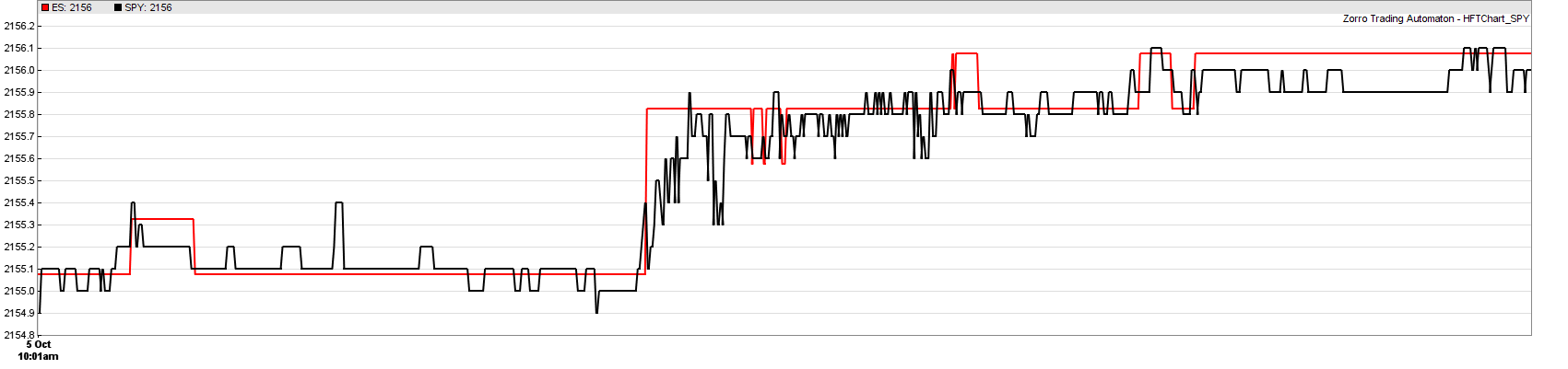
The resolution is 1 ms. ES is plotted in $ units, SPY in 10 cents units, with a small offset so that the curves lie over each other. The prices shown are ask prices. We can see that ES moves in steps of 25 cents, SPY in steps of 1 cent. The prices are still well correlated even on a millisecond scale. ES appears to trail a tiny bit.

We can also see an arbitrage opportunity at the steep price step in the center at about 10:01:30. ES reacted a bit slower, but stronger on some event, probably a moderate price jump of one of the stocks of the S&P 500. This event also triggered a fast sequence of oscillating SPY quotes, most likely from other HFT systems, until the situation calmed down again a few 100 ms later (the scale is not linear since time periods with no quotes are skipped). For several milliseconds the ES-SPY difference exceeded the ask-bid spread of both assets (usually 25 cents for ES and 1..4 cents for SPY). We would here ideally sell ES and buy SPY immediately after the ES price step. So we have verified that the theoretized inefficiency does really exist, at least in this sample. 

The script for displaying high resolution charts:

#define ES_HISTORY	"ES_201610.t1"
#define SPY_HISTORY	"SPY_201610.t1"
#define TIMEFORMAT	"%Y%m%d %H:%M:%S"
#define FACTOR		10
#define OFFSET		3.575

void main()
{
	var StartTime = wdatef(TIMEFORMAT,"20161005 10:01:25"),
		EndTime = wdatef(TIMEFORMAT,"20161005 10:01:35");
	MaxBars = 10000;
	BarPeriod = 0.001/60.;	// 1 ms plot resolution
	Outlier = 1.002;  // filter out 0.2% outliers

	assetList("HFT.csv");
	dataLoad(1,ES_HISTORY,2);
	dataLoad(2,SPY_HISTORY,2);
	int RowES=0, RowSPY=0;
	
	while(Bar < MaxBars)
	{
		var TimeES = dataVar(1,RowES,0), 
			PriceES = dataVar(1,RowES,1), 
			TimeSPY = dataVar(2,RowSPY,0), 
			PriceSPY = dataVar(2,RowSPY,1);

		if(TimeES < TimeSPY) RowES++;
		else RowSPY++;

		if(min(TimeES,TimeSPY) < StartTime) continue;
		if(max(TimeES,TimeSPY) > EndTime) break;

		if(TimeES < TimeSPY) {
			asset("ES");
			priceQuote(TimeES,PriceES);
		} else {
			asset("SPY");
			priceQuote(TimeSPY,PriceSPY);
		}
		
		asset("ES");
		if(AssetBar > 0) plot("ES",AskPrice+OFFSET,LINE,RED);
		asset("SPY");
		if(AssetBar > 0) plot("SPY",FACTOR*AskPrice,LINE,BLACK);
	}
}

The script first reads the two historical data files that we’ve created above, and then parses them row by row. For keeping the ES and SPY quotes in sync, we always read the quote with the smaller timestamp from the datasets (the quotes are stored in ascending timestamp order). The priceQuote function checks the prices for outliers, stores the ask price in the AskPrice variable and the ask-bid difference in Spread, and increases the Bar count for plotting the price curves. A bar of the curve is equivalent to 1 ms. The AssetBar variable is the last bar with a price quote of that asset, and is used here to prevent plotting before the first quote arrived. 

Testing the system

For backtesting our HFT system, we only need to modify the script above a bit, and call the tradeHFT function in the loop:

#define LATENCY		4.0	// milliseconds

function main()
{
	var StartTime = wdatef(TIMEFORMAT,"20161005 09:30:00"),
		EndTime = wdatef(TIMEFORMAT,"20161005 15:30:00");
	MaxBars = 200000;
	BarPeriod = 0.1/60.;	// 100 ms bars 
	Outlier = 1.002;

	assetList("HFT.csv");
	dataLoad(1,ES_HISTORY,2);
	dataLoad(2,SPY_HISTORY,2);
	int RowES=0, RowSPY=0;
	
	EntryDelay = LATENCY/1000.;
	Hedge = 2;
	Fill = 8; // HFT fill mode;
	Slippage = 0;
	Lots = 100;
		
	while(Bar < MaxBars)
	{
		var TimeES = dataVar(1,RowES,0), 
			PriceES = dataVar(1,RowES,1),
			TimeSPY = dataVar(2,RowSPY,0),
			PriceSPY = dataVar(2,RowSPY,1);

		if(TimeES < TimeSPY) RowES++;
		else RowSPY++;

		if(min(TimeES,TimeSPY) < StartTime) continue;
		if(max(TimeES,TimeSPY) > EndTime) break;

		if(TimeES < TimeSPY) {
			asset("ES");
			priceQuote(TimeES,PriceES);
		} else {
			asset("SPY");
			priceQuote(TimeSPY,FACTOR*PriceSPY);
		}
		
		asset("ES");
		if(!AssetBar) continue;
		var AskES = AskPrice, BidES = AskPrice-Spread;
		asset("SPY");
		if(!AssetBar) continue;
		var AskSPY = AskPrice, BidSPY = AskPrice-Spread;

		int Order = tradeHFT(AskSPY,BidSPY,AskES,BidES);	
		switch(Order) {
			case 1: 
			asset("ES"); enterLong();
			asset("SPY"); enterShort();
			break;
		
			case 2: 
			asset("ES"); enterShort();
			asset("SPY"); enterLong();
			break;
		
			case 0:
			asset("ES"); exitLong(); exitShort();
			asset("SPY"); exitLong(); exitShort();
			break;
		}
	}
	printf("\nProfit %.2f at NY Time %s",
		Equity,strdate(TIMEFORMAT,dataVar(1,RowES,0)));
}

This script runs a HFT backtest of one trading day, from 9:30 until 15:30 New York time. We can see that it just calls the HFT function with the ES and SPY prices, then executes the returned code in the switch-case statement. It opens 100 units of each asset (equivalent to 2 ES and 1000 SPY contracts). The round-trip latency is set up with the EntryDelay variable. In HFT mode (Fill = 8), a trade is filled at the most recent price quote after the given delay. This ensures a realistic latency simulation when price quotes are entered with their exchange time stamps.

Here’s the HFT profit at the end of the day with different round-trip latency values:

LATENCY	0.5 ms	4.0 ms	6.0 ms	10 ms
Profit / day	+ $793	+ $273	+ $205	– $15

The ES-SPY HFT arbitrage system makes about $800 each day with an unrealistic small latency of 500 microseconds. Unfortunately, due to the 700 miles between the NYSE and the CME, you’d need a time machine for that (or some faster-than-light method of quantum teleportation). A HFT server in Warren, Ohio, at 4 ms latency would generate about $300 per day. A server slightly off the direct NY-Chicago line can still grind out $200 daily. But the system deteriorates quickly when located further away, as with a server in Nashville, Tennessee, at around 10 ms latency. This is a strong hint that some high-speed systems in the proximity of both exchanges are already busy with exploiting ES-SPY arbitrage.

Still, $300 per day result in a decent $75,000 annual income. However, what needed you to invest for that, aside from hardware and software? With SPY at $250, the 100 units translate to 100*$2500 + 100*10*$250 = half a million dollars trade volume. So you would get only 15% annual return on your investment. But you can improve this by adding more pairs of NY ETFs and their equivalent CME futures to the arbitrage strategy. And you can improve it further when you find a broker or similar service that can receive your orders directly at the exchanges. Due to the ETF/future hedging the position is almost without risk. So you could probably negotiate a large leverage. And also a flat monthly fee, since broker commissions were not included in the test.

Conclusion 

• When systems react fast enough, profits can be achieved with very primitive methods, such as arbitrage between highly correlated assets.
• Location has a large impact on HFT profits.
• ES-SPY arbitrage cannot be traded by everyone from everywhere. You’re competing with people that are doing this already. Possibly in Warren, Ohio.

I’ve added the scripts and the asset list to the 2017 script archive in the “HFT” and “History” folders. Unfortunately I could not add the ES / SPY price history files, since I do not own the data. For reproducing the results, get BBO history from Nanex™ or Nanotick™ – their data can be read with the scripts above. You’ll also need Zorro S version 1.60 or above, which supports HFT fill mode.

References

(1) When Correlations Break Down (Jared Bernstein 2014)

(2) Financial Programming Greatly Accelerated (Cousin/Weston, Automated Trader 42/2017)

 

---

Addendum. I have been asked how the profit would be affected when the server is located in New York, with 0.25 ms signal delay to the NYSE and 4.8 ms signal delay to the CME. For simulating this, modify the script:

var TimeES = dataVar(1,RowES,0)+4.8/(1000*60*60*24),
  TimeSPY = dataVar(2,RowSPY,0)+0.25/(1000*60*60*24),
...
switch(Order) {
	case 1: 
		EntryDelay = 4.8/1000;
		asset("ES"); enterLong();
		EntryDelay = 0.25/1000;
		asset("SPY"); enterShort();
		break;
		
	case 2: 
		EntryDelay = 4.8/1000;
		asset("ES"); enterShort();
		EntryDelay = 0.25/1000;
		asset("SPY"); enterLong();
		break;
		
	case 0:
		EntryDelay = 4.8/1000;
		asset("ES"); exitLong(); exitShort();
		EntryDelay = 0.25/1000;
		asset("SPY"); exitLong(); exitShort();
		break;
}

The first line simulates the price quote arrivals with 4.8 and 0.25 ms delay, the other lines establish the different order delays for SPY and ES. Alternatively, you could artificially delay the incoming SPY quotes by another 4.55 ms, so that their time stamps again match the ES quotes. In both cases the system returns about $240 per day, almost as much as in Warren. However a similar system located in Aurora, close to Chicago (swap the delays in the script), would produce zero profit. The asymmetry is caused by the relatively long constant periods of ES, making the SPY latency more relevant for the money at the end of the day.