Petra on Programming: A Unique Trend Indicator

This months project is a new indicator by John Ehlers, first published in the S&C May 2020 issue. Ehlers had a unique idea for early detecting trend in a price curve. No smoothing, no moving average, but something entirely different. Lets see if this new indicator can rule them all.

The basic idea of the Correlation Trend Indicator (CTI) is quite simple. The ideal trend curve is a straight upwards line. So the CTI just measures the correlation of the price curve with this ideal trend line. Ehlers provided TradeStation code that can be directly converted to Zorro’s C language. This is the indicator:

var CTI (vars Data, int Length)
{
  int count;
  var Sx = 0, Sy = 0, Sxx = 0, Sxy = 0, Syy = 0;
  for(count = 0; count < Length; count++) {
    var X = Data[count]; // the price curve
    var Y = -count; // the trend line
    Sx = Sx + X; Sy = Sy + Y;
    Sxx = Sxx + X*X; Sxy = Sxy + X*Y; Syy = Syy + Y*Y;
  }
  if(Length*Sxx-Sx*Sx > 0 && Length*Syy-Sy*Sy > 0)
    return (Length*Sxy-Sx*Sy)/sqrt((Length*Sxx-Sx*Sx)*(Length*Syy-Sy*Sy));
  else return 0;
}

X represents the price curve, Y the trend line, and correlation is measured with the Spearman algorithm. The trend line is supposed to linearly rise with count, but I’m using the negative count here because the Data series is stored backwards, with the most recent values at the begin.

This is how the CTI looks when applied to SPY (red = 10 days period, blue = 40 days):

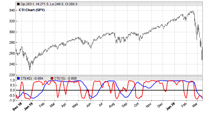
We can see that the lines reproduce rather well the price curve trend. And we can also see that the blue line, the 40-days trend, is not just a smoothed version of the red 10-days trend – it looks entirely different. This is an interesting feature of a trend indicator – it separates long-term and short-term trend perfectly. But does the indicator have predictive power?

For finding out, we could use it for a simple trading system. But a bit more informative is examining a price difference profile of its zero crossovers. A price difference profile displays the average price movement and its standard deviation for the bars following a certain event or condition. It is used for testing the quality of trade signals.

The code for plotting a price difference profile from the CTI(20) zero crossings:

void run() 
{
   BarPeriod = 1440;
   LookBack = 40;
   StartDate = 2010;

   assetAdd("SPY","STOOQ:SPY.US"); // load SPY history from Stooq
   asset("SPY");

   vars Prices = series(priceClose());
   vars Signals = series(CTI(Prices,20));
   if(crossOver(Signals,0))
      plotPriceProfile(40,0); // plot positive price difference
   else if(crossUnder(Signals,0))
      plotPriceProfile(40,2); // plot negative price difference
}

The resulting profile:

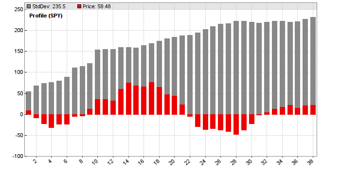
The red bars are the average differences (in cents) to the price at the zero crossings. The X axis shows the days after the crossing.

We can see that the average price differences tend to drop to a negative minimum immediately after a crossing, thus indicating a short term mean reversion effect. Then the differences rise to a trend maximum after about 14 days. The effect is trend neutral by including negative differences at reverse crossings. The optimal trading system for this profile would be entering a long or short position 4 days after the CTI crossing, then holding the position for 10 days. 

But we can also see that the standard deviation of the price differences – the grey bars, reduced by factor 4 for better scaling – is about ten times higher than the price difference extrema. So the effect is small, and trading on CTI crossovers would be difficult. A somewhat predictive power of the CTI(SPY,20) exists – but it is too weak for being directly exploited in a crossover trading system.

Reference

John Ehlers, Correlation Trend Indicator, Stocks&Commodities 5/2020

The indicator and price profile test scripts are available in the Scripts 2020 repository.