About 9 out of 10 backtests produce wrong or misleading results. This is the number one reason why carefully developed algorithmic trading systems often fail in live trading. Even with out-of-sample data and even with cross-validation or walk-forward analysis, backtest results are often way off to the optimistic side. The majority of trading systems with a positive backtest are in fact unprofitable. In this article I’ll discuss the cause of this phenomenon, and how to fix it.
Suppose you’re developing an algorithmic trading strategy, following all rules of proper system development. But you are not aware that your trading algorithm has no statistical edge. The strategy is worthless, the trading rules equivalent to random trading, the profit expectancy – aside from transaction costs – is zero. The problem: you will rarely get a zero result in a backtest. A random trading strategy will in 50% of cases produce a negative backtest result, in 50% a positive result. But if the result is negative, you’re normally tempted to tweak the code or select assets and time frames until you finally got a profitable backtest. Which will happen relatively soon even when applying random modifications to the system. That’s why there are so many unprofitable strategies around, with nevertheless great backtest performances.
Does this mean that backtests are worthless? Not at all. But it is essential to know whether you can trust the test, or not.
The test-the-backtest experiment
There are several methods for verifying a backtest. None of them is perfect, but all give insights from different viewpoints. We’ll use the Zorro algo trading software, and run our experiments with the following test system that is optimized and backtested with walk-forward analysis:
function run()
{
  set(PARAMETERS,TESTNOW,PLOTNOW,LOGFILE);
  BarPeriod = 1440;
  LookBack = 100;
  StartDate = 2012;
  NumWFOCycles = 10;

  assetList("AssetsIB");
  asset("SPY");

  vars Signals = series(LowPass(seriesC(),optimize(10,2,20,2)));
  vars MMIFast = series(MMI(seriesC(),optimize(50,40,60,5)));
  vars MMISlow = series(LowPass(MMIFast,100));

  MaxLong = 1;
  if(falling(MMISlow)) {
    if(valley(Signals))
      enterLong();
    else if(peak(Signals))
      exitLong();
  }
}
This is a classic trend following algorithm. It uses a lowpass filter for trading at the peaks and valleys of the smoothed price curve, and a MMI filter (Market Meanness Index) for distinguishing trending from non-trending market periods. It only trades when the market has switched to rend regime, which is essential for profitable trend following systems. It opens only long positions. Lowpass and MMI filter periods are optimized, and the backtest is a walk-forward analysis with 10 cycles.
The placebo trading system
It is standard for experiments to compare the real stuff with a placebo. For this we’re using a trading system that has obviously no edge, but was tweaked with the evil intention to appear profitable in a walk-forward analysis. This is our placebo system:
void run()
{
  set(PARAMETERS,TESTNOW,PLOTNOW,LOGFILE);
  BarPeriod = 1440;
  StartDate = 2012;
  setf(TrainMode,BRUTE);
  NumWFOCycles = 9;

  assetList("AssetsIB");
  asset("SPY");

  int Pause = optimize(5,1,15,1);
  LifeTime = optimize(5,1,15,1);

// trade after a pause...
  static int NextEntry;
  if(Init) NextEntry = 0;
  if(NextEntry-- <= 0) {
    NextEntry = LifeTime+Pause;
    enterLong();
  }
}
This system opens a position, keeps it a while, then closes it and pauses for a while. The trade and pause durations are walk-forward optimized between 1 day and 3 weeks. LifeTime is a predefined variable that closes the position after the given time. If you don’t believe in lucky trade patterns, you can rightfully assume that this system is equivalent to random trading. Let’s see how it fares in comparison to the trend trading system.
Trend trading vs. placebo trading
This is the equity curve with the trend trading system from a walk forward analysis from 2012 up to 3/2022:
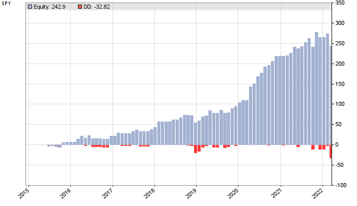
The plot begins 2015 because the preceding 3 years are used for the training and lookback periods. SPY follows the S&P500 index and rises in the long term, so we could expect anyway some profit with a long-only system. But this system, with profit factor 3 and R2 coefficient 0.65 appears a lot better than random trading. Let’s compare it with the placebo system:
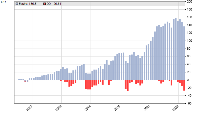
The placebo system produced profit factor 2 and R2 coefficient 0.77. Slightly less than the real system, but in the same performance range. And this result was also from a walk-forward analysis, although with 9 cycles – therefore the later start of the test period. Aside from that, it seems impossible to determine solely from the equity curve and performance data which system is for real, and which is a placebo.
Checking the reality
Methods to verify backtest results are named ‘reality check’. They are specific to the asset and algorithm; in a multi-asset, multi-algo portfolio, you need to enable only the component you want to test. Let’s first see how the WFO split affects the backtest. In this way we can find out whether our backtest result was just due to lucky trading in a particular WFO cycle. We’re going to plot a WFO profile that displays the effect of the number of walk-forward cycles on the result. For this we outcomment the NumWFOCycles = … line in the code, and run it in training mode with the WFOProfile.c script:
#define run strategy
#include "trend.c" // <= your script
#undef run
#define CYCLES 20 // max WFO cycles

function run()
{
  set(TESTNOW);
  NumTotalCycles = CYCLES-1;
  NumWFOCycles = TotalCycle+1;
  strategy();
}

function evaluate()
{
  var Perf = ifelse(LossTotal > 0,WinTotal/LossTotal,10);
  if(Perf > 1)
    plotBar("WFO+",NumWFOCycles,NumWFOCycles,Perf,BARS,BLACK);
  else
    plotBar("WFO-",NumWFOCycles,NumWFOCycles,Perf,BARS,RED);
}
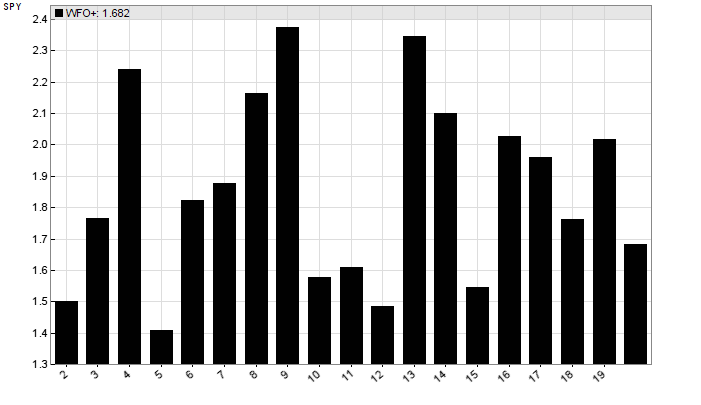
We’re redefining the run function to a different name. This allows us to just include the tested script and train it with WFO cycles from 2 up to the number defined by CYCLES. A backtest is executed after training. If an evaluate function is present, Zorro runs it automatically after any backtest. It plots a histogram bar of the profit factor (y axis) from each number of WFO cycles. First, the WFO profile of the trend trading system:
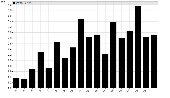
We can see that the performance rises with the number of cycles. This is typical for a system that adapts to the market. All results are positive with a profit factor > 1. Our arbitrary choice of 10 cycles produced a less than average result. So we can at least be sure that this backtest result was not caused by a particularly lucky number of WFO cycles.
The WFO profile of the placebo system:
This time the number of WFO cycles had a strong random effect on the performance. And it is now obvious why I used 9 WFO cycles for that system. For the same reason I used brute force optimization, since it increases WFO variance and thus the chance to get lucky WFO cycle numbers. That’s the opposite of what we normally do when developing algorithmic trading strategies.
WFO profiles give insight into WFO cycle dependency, but not into randomness or overfitting by other means. For this, more in-depth tests are required. Zorro supports two methods, the Montecarlo Reality Check (MRC) with randomized price curves, and White’s Reality Check (WRC) with detrended and bootstrapped equity curves of strategy variants. Both methods have their advantages and disadvantages. But since strategy variants from optimizing can only be created without walk-forward analysis, we’re using the MRC here.
The Montecarlo Reality Check
First we test both systems with random price curves. Randomizing removes short-term price correlations and market inefficiencies, but keeps the long-term trend. Then we compare our original backtest result with the randomized results. This yields a p-value, a metric of the probability that our test result was caused by randomness. The lower the p-Value, the more confidence we can have in the backtest result. In statistics we normally consider a result significant when its p-Value is below 5%.
The basic algorithm of the Montecarlo Reality Check (MRC):
- Train your system and run a backtest. Store the profit factor (or any other performance metric that you want to compare).
- Randomize the price curve by randomly swapping price changes (shuffle without replacement).
- Train your system again with the randomized data and run a backtest. Store the performance metric.
- Repeat steps 2 and 3 1000 times.
- Determine the number N of randomized tests that have a better result than the original test. The p-Value is N/1000.
If our backtest result was affected by an overall upwards trending price curve, which is certainly the case for this SPY system, the randomized tests will be likewise affected. The MRC code:
#define run strategy
#include "trend.c" // <= your script
#undef run
#define CYCLES 1000

function run()
{
  set(PRELOAD,TESTNOW);
  NumTotalCycles = CYCLES;
  if(TotalCycle == 1) // first cycle = original
    seed(12345); // always same random sequence
  else
    Detrend = SHUFFLE;
  strategy();
  set(LOGFILE|OFF); // don't export files
}

function evaluate()
{
  static var OriginalProfit, Probability;
  var PF = ifelse(LossTotal > 0,WinTotal/LossTotal,10);
  if(TotalCycle == 1) {
    OriginalProfit = PF;
    Probability = 0;
  } else {
    if(PF < 2*OriginalProfit) // clip image at double range
      plotHistogram("Random",PF,OriginalProfit/50,1,RED);
    if(PF > OriginalProfit)
      Probability += 100./NumTotalCycles;
  }
  if(TotalCycle == NumTotalCycles) { // last cycle
    plotHistogram("Original",
     OriginalProfit,OriginalProfit/50,sqrt(NumTotalCycles),BLACK);
    printf("\n-------------------------------------------");
    printf("\nP-Value %.1f%%",Probability);
    printf("\nResult is ");
    if(Probability <= 1)
      printf("highly significant") ;
    else if(Probability <= 5)
      printf("significant");
    else if(Probability <= 15)
      printf("maybe significant");
    else
      printf("statistically insignificant");
    printf("\n-------------------------------------------");
  }
}
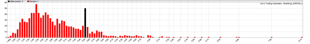
This code sets up the Zorro platform to train and test the system 1000 times. The seed setting ensures that you get the same result on any MRC run. From the second cycle on, the historical data is shuffled without replacement. For calculating the p-value and plotting a histogram of the MRC, we use the evaluate function again. It calculates the p-value by counting the backtests resulting in higher profit factors than the original system. Depending on the system, training and testing the strategy a thousand times will take several minutes with Zorro. The resulting MRC histogram of the trend following system:
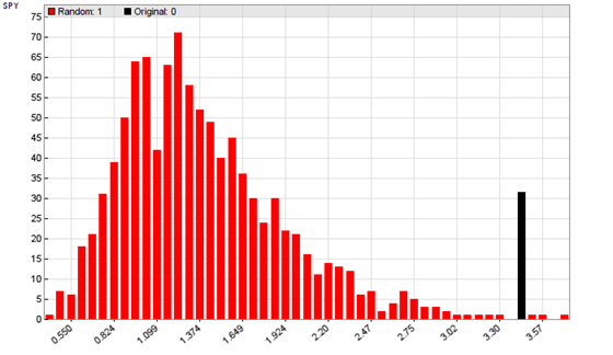
The height of a red bar represents the number of shuffled backtests that ended at the profit factor shown on the x axis. The black bar on the right (height is irrelevant, only the x axis position matters) is the profit factor with the original price curve. We can see that most shuffled tests came out positive, due to the long-term upwards trend of the SPY price. But our test system came out even more positive. The p-Value is below 1%, meaning a high significance of our backtest. This gives us some confidence that the simple trend follower can achieve a similar result in real trading.
This cannot be said from the MRC histogram of the placebo system:
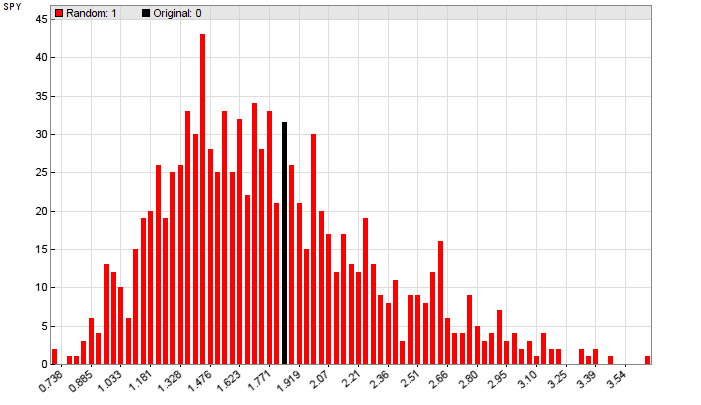
The backtest profit factors now extend over a wider range, and many were more profitable than the original system. The backtest with the real price curve is indistinguishable from the randomized tests, with a p-value in the 40% area. The original backtest result of the placebo system, even though achieved with walk-forward analysis, is therefore meaningless.
It should be mentioned that the MRC cannot detect all invalid backtests. A system that was explicitly fitted to a particular price curve, for instance by knowing in advance its peaks and valleys, would get a low p-value by the MRC. No reality check could distinguish such a system from a system with a real edge. Therefore, neither MRC nor WRC can give absolute guarantee that a system works when it passes the check. But when it does not pass, you’re advised to better not trade it with real money.
I have uploaded the strategies to the 2022 script repository. The MRC and WFOProfile scripts are included in Zorro version 2.47.4 and above. You will need Zorro S for the brute force optimization of the placebo system.
Any binary system that goes full long or full short, nothing in between (except going flat), is subject to overfitting. Period.
Why do you think non-binary systems are less likely to overfit? Question mark.
A good read. Although ain’t seeing “magic pill” on a quick glance. Not for me at least. Maybe after couple re-reads and some time.
My experience is that the trading system that produces trading signals at peaks and valleys both during the optimization period and out-of-sample data period last longer.
The problem with backtesting is , the variety or the range that you capture could be so old as to be useless tomorrow.So how to capture the same or similar profitable range?
May be predictive conditional indicators are necessary to signify the presence or absence of range conditions.Conditional indicators showing the highest value and lowest value within a certain number of bars. Or number of bars specified and appears in a chart etc..Then again in my opinion ,self learning machine learning algorithms are necessary.
I always appreciate your interesting articles. Still, in this matter, under my experience, I watch that markets are always breaking patterns. It doesn’t matter how well you can fit your model, eventually, it’ll go out of service for a while. And I’m not even talking about other factors such as executions, frequency..etc I always end up with a daily (kind of slow mode) trading as the sweet time frame for me, and still a big challenge every day.
I am following the steps and examples above to try to run the WFOProfile.c to generate WFO profile for the trend.c script but could not get it working. Both the trend.c and WFOProfile.c scripts remain unchanged as shown above. The #include line in the WFOProfile.c still points to “trend.c”. When I run the WFOProfile.c script in the training mode, I got this error:
WFOProfile compiling..
Error in ‘trend.c’ line 1:
‘function’ undeclared identifier
.
Could you please point out what I might did wrong? Thanks.
Update: instead of using the code example above for the WFOProfile.c, I used the script that is included with Zorro and it is working. However, the WFO profile I got looks different from that posted above. The profile has a somewhat random look to it rather than a gradual rising in slope. The only modification I did is to add the line below to the trend.c script.
EndDate = 2022;
This end date is added so that the data range used in this training is consistent with that used to produce the WFO profile above – namely the data spans from 2012-2022. I could not seem to attach an image here. Instead, I will list the approximate values of the profit factors for the range of number of WFO cycles.
2: 3.5
3: 1.2
4: 2.05
5: 1.65
6: 2.1
7: 1.9
8: 1.85
9: 2.5
10: 1.85
11: 1.75
12: 1.7
13: 2.95
14: 3.2
15: 2.0
16: 1.8
17: 2.05
18: 2.9
19: 2.4
20: 2.1
What can cause the differences in the two WFO profiles? Thanks.
There can be lots of reasons. I can hardly tell what it is, for this I had to examine your code, but Zorro support can do that and answer questions of this kind.
When do you use the bootstrap mode, f.i.
Detrend = BOOTSTRAP;
It seems this method generates a set of new price curves that might or might not have any anomalies. Thanks.
BOOTSTRAP is used for generating random curves with different end results. SHUFFLE is used when you want the same end results.
Can the Montecarlo Reality Check (MRC.c) simulation time be speeded up? for example, with the use of multi-cores (NumCores = -1)? Thank you.
Sure, a MRC with WFO training can use multiple cores and run accordingly faster.
On the 1st paragraph of page 138 in the Black Book, you mentioned that during MRC run with the use of Detrend = SHUFFLE, TRAIN mode is not needed to repeat thousands of times when using WFO. The mentioned reason for this is because it does not matter whether training was done with shuffled data or with original data. Why does it not matter? Thanks.
Only for this system. With other systems, it can very well matter.
The system is based on the assumption that 3-candle patterns in the training data also occur in the test data. Since shuffling replaces these pattern with random patterns, it destroys any correlation between test and training patterns. It does not matter if one of them remains original, or is also shuffled.
What I tried to do is this:
1. in the MRC file, set the CYCLES parameter to 1, i.e.,
#define CYCLES 1
2. clicked on [Train]. Training is done with original data
3. set the CYCLES parameter back to 1000, i.e.,
#define CYCLES 1000
4. clicked on [Test]
The RANDOMIZE parameter is set to SHUFFLE. Are the above steps valid for performing a MRC test? Thanks.
In a porfolio system, would it be possible to have multiple and different number of WFO cycles (NumWFOCycles) for different symbols? f.i., symbol A has NumWFOCycles = 5, while symbol B has NumWFOCycles=10? If so, how would you do it? Thank you.
No, the WFO period is the same for all assets.
In a portfolio system, do I have to do the MRC for each component separately or can I do the MRC with all de components of the portfolio at the same time? Thank you.
You can do both, but normally it’s for all components.